Mechanistic-Empirical Pavement Design Model: Enhancements of Climatic Inputs (2025)
Chapter: 3 Interpretations and Applications
CHAPTER 3
Interpretations and Applications
The enhancements developed to address the limitations identified in Chapter 2 are discussed in detail in this chapter, which includes the following major sections:
- Improving and Simplifying the Climate Input Parameters for Pavement ME
- Developing Enhancements of Climatic Inputs and Related Models for Future Incorporation in Pavement ME Design
- Validating New or Enhanced Models
- Identifying Enhancements to Improve EICM Functionality and Maintainability
3.1 Improving and Simplifying the Climate Input Parameters for Pavement ME
The LTPP InfoPave Climate Tool only includes a subset of the complete MERRA-2 dataset. The objectives of this task are to identify the MERRA-2 variables not included in the LTPP InfoPave Climate Tool that may be applicable for pavement applications, extract a representative subset for extensive testing, and provide recommendations on which variables to include that can simplify or enhance the EICM predictions. This section is structured as follows:
- A listing of available MERRA-2 data tables applicable to pavements
- A summary of MERRA-2 data extraction and unit conversions
- A selected set of comparisons and final variable selections
- A proposed process to integrate selected variables into the LTPP InfoPave Climate Tool
3.1.1 Available MERRA-2 Data Tables and Variables for Pavement Applications
The MERRA-2 NASA data tables with hourly data for potential use in pavement applications include the radiation diagnostics (tavg1_2d_rad_Nx), land surface diagnostics (tavg1_2d_lnd_ Nx), vertically integrated diagnostics (tavg1_2d_int_Nx), surface flux diagnostics (tavg1_2d_ flx_Nx), single-level diagnostics (inst1_2d_asm_Nx), and constant land–surface parameters (const_2d_lnd_Nx) tables (12). The shortlisted variables, which may have pavement applications, are summarized in Tables 2 through 6. It should be noted that in Table 2, the SPEED and SPEEDMAX descriptions are identical while their names are different. The MERRA-2 documentation does not specify a difference while it is suspected that the SPEEDMAX represents the maximum hourly wind speed.
Table 2. List of surface flux diagnostics (tavg1_2d_flx_Nx) variables for potential pavement applications.
| Name | Description | Units (SI) | U.S. Equivalent Units |
|---|---|---|---|
| PRECSNO | Snowfall | kg m–2 s–1 | lb ft–2 s–1 |
| PRECTOT | Total precipitation from atmospheric model physics | kg m–2 s–1 | lb ft–2 s–1 |
| PRECTOTCORR | Bias corrected total precipitation | kg m–2 s–1 | lb ft–2 s–1 |
| RHOA | Air density at surface | kg m–3 | lb ft–3 |
| TLML | Surface air temperature | K | K |
| ULML | Surface eastward wind | m s–1 | mi h–1 |
| VLML | Surface northward wind | m s–1 | mi h–1 |
| EFLUX | Total latent energy flux | W m–2 | BTU ft–2 h–1 |
| SPEED | Surface wind speed | m s–1 | mi h–1 |
| SPEEDMAX | Surface wind speed | m s–1 | mi h–1 |
Table 3. List of land surface diagnostics (tavg1_2d_lnd_Nx) variables for potential pavement applications.
| Name | Description | Units (SI) | U.S. Equivalent Units |
|---|---|---|---|
| EVLAND | Evaporation land | kg m–2 s–1 | lb ft–2 s–1 |
| EVPTRNS | Transpiration energy flux | W m–2 | BTU ft–2 h–1 |
| LWLAND | Net longwave land | W m–2 | BTU ft–2 h–1 |
| QINFIL | Soil water infiltration rate | kg m–2 s–1 | lb ft–2 s–1 |
| RUNOFF | Overland runoff, including throughflow | kg m–2 s–1 | lb ft–2 s–1 |
| SMLAND | Snowmelt flux land | kg m–2 s–1 | lb ft–2 s–1 |
| SWLAND | Net shortwave land | W m–2 | BTU ft–2 h–1 |
| TSAT | Surface temperature of saturated zone | K | K |
| TSOIL1 | Soil temperatures layer 1 | K | K |
| TSOIL2 | Soil temperatures layer 2 | K | K |
| TSOIL3 | Soil temperatures layer 3 | K | K |
| TSOIL4 | Soil temperatures layer 4 | K | K |
| TSOIL5 | Soil temperatures layer 5 | K | K |
| TSOIL6 | Soil temperatures layer 6 | K | K |
| TUNST | Surface temperature of unsaturated zone | K | K |
| ECHANGE | Rate of change of total land energy | W m–2 | BTU ft–2 h–1 |
| GHLAND | Ground heating land | W m–2 | BTU ft–2 h–1 |
| LHLAND | Latent heat flux land | W m–2 | BTU ft–2 h–1 |
| PRECTOTLAND | Total precipitation land; bias corrected | kg m–2 s–1 | lb ft–2 s–1 |
| SHLAND | Sensible heat flux land | W m–2 | BTU ft–2 h–1 |
| SPLAND | Rate of spurious land energy source | W m–2 | BTU ft–2 h–1 |
| SPSNOW | Rate of spurious snow energy | W m–2 | BTU ft–2 h–1 |
| TPSNOW | Surface temperature of snow | K | K |
| TSURF | Surface temperature of land, including snow | K | K |
Table 4. List of constant land–surface parameters (const_2d_lnd_Nx) variables for potential pavement applications.
| Name | Description | Units (SI) | U.S. Equivalent Units |
|---|---|---|---|
| dzgt1 | Thickness of soil layer associated with TSOIL1 | m | ft or in |
| dzgt2 | Thickness of soil layer associated with TSOIL2 | m | ft or in |
| dzgt3 | Thickness of soil layer associated with TSOIL3 | m | ft or in |
| dzgt4 | Thickness of soil layer associated with TSOIL4 | m | ft or in |
| dzgt5 | Thickness of soil layer associated with TSOIL5 | m | ft or in |
| dzgt6 | Thickness of soil layer associated with TSOIL6 | m | ft or in |
| poros | Soil porosity in volumetric units | m–3 m–3 | ft–3 ft–3 |
Table 5. List of vertically integrated diagnostics (tavg1_2d_int_Nx) variables for potential pavement application.
| Name | Description | Units (SI) | U.S. Equivalent Units |
|---|---|---|---|
| LWGNET | Surface net downward longwave flux | W m–2 | BTU ft–2 h–1 |
| LWTNET | Upwelling longwave flux at top of the atmosphere (TOA) | W m–2 | BTU ft–2 h–1 |
| PRECLS | Large scale rainfall | kg m–2 s–1 | lb ft–2 s–1 or in |
| SWNETSRF | Surface net downward shortwave flux | W m–2 | BTU ft–2 h–1 |
| SWNETTOA | TOA net downward shortwave flux | W m–2 | BTU ft–2 h–1 |
| HFLUX | Sensible heat flux from turbulence | W m–2 | BTU ft–2 h–1 |
Table 6. List of radiation diagnostics (tavg1_2d_rad_Nx) variables for potential pavement applications.
| Name | Description | Units (SI) | U.S. Equivalent Units |
|---|---|---|---|
| ALBEDO | Surface albedo | 1 | 1 |
| CLDHGH | Cloud area fraction for high clouds | 1 | 1 |
| CLDLOW | Cloud area fraction for low clouds | 1 | 1 |
| CLDMID | Cloud area fraction for middle clouds | 1 | 1 |
| CLDTOT | Total cloud area fraction | 1 | 1 |
| EMIS | Surface emissivity | 1 | 1 |
| LWGAB | Surface absorbed longwave radiation | W m–2 | BTU ft–2 h–1 |
| LWGABCLR | Surface absorbed longwave radiation assuming clear sky | W m–2 | BTU ft–2 h–1 |
| LWGABCLRCLN | Surface absorbed longwave radiation assuming clear sky and no aerosol | W m–2 | BTU ft–2 h–1 |
| LWGEM | Longwave flux emitted from surface | W m–2 | BTU ft–2 h–1 |
| LWGNT | Surface net downward longwave flux | W m–2 | BTU ft–2 h–1 |
| Name | Description | Units (SI) | U.S. Equivalent Units |
|---|---|---|---|
| LWGNTCLR | Surface net downward longwave flux assuming clear sky | W m–2 | BTU ft–2 h–1 |
| LWGNTCLRCLN | Surface net downward longwave flux assuming clear sky and no aerosol | W m–2 | BTU ft–2 h–1 |
| LWTUP | Upwelling longwave flux at TOA | W m–2 | BTU ft–2 h–1 |
| LWTUPCLR | Upwelling longwave flux at TOA assuming clear sky | W m–2 | BTU ft–2 h–1 |
| LWTUPCLRCLN | Upwelling longwave flux at TOA assuming clear sky and no aerosol | W m–2 | BTU ft–2 h–1 |
| SWGDN | Surface incoming shortwave flux | W m–2 | BTU ft–2 h–1 |
| SWGDNCLR | Surface incoming shortwave flux assuming clear sky | W m–2 | BTU ft–2 h–1 |
| SWGNT | Surface net downward shortwave flux | W m–2 | BTU ft–2 h–1 |
| SWGNTCLN | Surface net downward shortwave flux assuming no aerosol | W m–2 | BTU ft–2 h–1 |
| SWGNTCLR | Surface net downward shortwave flux assuming clear sky | W m–2 | BTU ft–2 h–1 |
| SWGNTCLRCLN | Surface net downward shortwave flux assuming clear sky and no aerosol | W m–2 | BTU ft–2 h–1 |
| SWTDN | TOA incoming shortwave flux | W m–2 | BTU ft–2 h–1 |
| SWTNT | TOA net downward shortwave flux | W m–2 | BTU ft–2 h–1 |
| SWTNTCLN | TOA net downward shortwave flux assuming no aerosol | W m–2 | BTU ft–2 h–1 |
| SWTNTCLR | TOA net downward shortwave flux assuming clear sky | W m–2 | BTU ft–2 h–1 |
| SWTNTCLRCLN | TOA net downward shortwave flux assuming clear sky and no aerosol | W m–2 | BTU ft–2 h–1 |
| TS | Surface skin temperature | K | K |
3.1.1.1 Summary of Unit Conversions
The MERRA-2 assimilated data are distributed in SI units, which may or may not require additional conversions to match those required by the EICM. Table 7 summarizes the unit conversions for the most common variables. The conversions listed in Table 7 were used throughout the analysis procedures in the subsequent tasks.
3.1.2 MERRA-2 Data Extraction and Evaluation
3.1.2.1 Data Extraction: Downloading MERRA-2 Data
MERRA-2 includes recent upgrades to the atmospheric assimilation, which enable the use of newer satellite observations that could not be assimilated in the original MERRA system. Additionally, MERRA-2 benefits from advances in the Goddard EOS, version 5 (GEOS-5) Atmospheric General Circulation Model (AGCM). MERRA-2 covers the period from 1980 to the present and continues to be updated with latency on the order of weeks. The AGCM is run on a cube-sphere grid with an approximate resolution of 50 km × 50 km, the atmospheric analysis operates on a Gaussian grid of the same resolution, and the output fields are interpolated to a
Table 7. Summary of units and conversion factors between MERRA-2 data and the EICM requirements.
| Variable Name | MERRA-2 Units | U.S. Customary | EICM Requirement | Conversion |
|---|---|---|---|---|
| Heat Flux Density | W/m2 | BTU/h-ft2 | BTU/h-ft2 | 1 W/m2 = 0.317 BTU/h-ft2 |
| Temperature | K | °F | °F or °C | 1 K = –457.87 °F, 1 K = –272.15 °C |
| Rainfall/Precipitation | kg m–2 s–1 | lb ft–2 s–1 | in or mm | Density of water = 1,000 kg m–3 1 kg m–2 = 1 mm of water 1 kg m–2 s–1 = 1 mm s–1 1 h = 60 min = 3,600 s 1 kg m–2 s–1 * 3,600 s = mm/h |
0.5° × 0.625° regular latitude–longitude grid prior to publication. For this research, the MERRA-2 variables listed in Tables 2 through 6 were extracted for a representative set of geographical locations covering the typical climatic regions, based on temperature and moisture, throughout the United States, as shown in Figure 1.
While the NASA Goddard Earth Sciences (GES) Data and Information Services Center (DISC) provides a web tool for sub-selecting and downloading the MERRA-2 database, it is a manual process and still requires the user to be able to know how to appropriately access and download needed data from the various data libraries and tables. The research team investigated multiple ways to work with GES DISC data resources using Python and open-source libraries, such as Request, Pydap, Xarray, and netCDF4-python. The Pydap library was chosen for this research project and is described as a convenient Python library that provides access to GES DISC OPeNDAP resources. It offers an interface for Python programs to read from OPeNDAP servers and also utilizes the netCDF4-Python module, which leverages the netCDF-C library to access the data. A MERRA-2 data download module using Pydap was developed, which requires authorized registration with GES DISC to download the data. Additionally, as described earlier, five different datasets were utilized to extract the climate variables for the 67 locations with different climate zones across the continental United States. Therefore, a total of 268 data tables were created to store all potential variables for each location. It should be mentioned that several limitations or issues were encountered that delayed the extraction process slightly. The main limitation was due to a “connection time exceeded” error that often occurred when attempting to download data over too many days because the server was receiving multiple requests from many users. The expected connection time to the server was approximately 2.5 h at a time. To overcome this problem, only the data corresponding to the grid covering the selected 67 locations were accessed and extracted. Additionally, the amount of data downloaded at one time was segmented to reduce processing and connection time to server.
3.1.2.2 Data Evaluation
Many of the datasets or data tables include similarly named variables. For example, net longwave and shortwave radiation data are included in the Flux, Radiation, and Land datasets, which may or may not be equivalent. Similarly named variables within each dataset were identified and compared to determine whether they are similar or different from one another. A brief description of one of the differences between the Flux and Land dataset collections is provided here (13):
WHAT IS THE DIFFERENCE BETWEEN FLUX DATA INCLUDED IN THE FLX COLLECTION AND THE LND COLLECTION?
MERRA’s land parameterization is Randy Koster’s Catchment model, but other surfaces, such as inland water, ocean surface and glaciers are also accounted for as sub-grid tiles. In the LND collection of variables, all the data are derived from the land model, and are not weighted according to the land fraction at that grid point. This data is provided to better compute land budgets for soil water and land energy.

The data in FLX, RAD or any other collection of variables represent the gridbox average of all the different tiles weighted by their fractional cover. This is where you would use evaporation to compute the atmospheric energy balance. The important distinction here is that LND is land only, while all other collections are representative of the whole grid box.
The common variables identified between the MERRA-2 datasets were analyzed to determine whether they correlated with one another. The results from the analysis will help determine the recommended final list of variables for inclusion in the LTPP InfoPave Climate Tool database. The comparisons focused on the longwave, shortwave, and total net radiation at the Earth’s surface.
The dataset names were renamed to help make them more descriptive and easily identifiable. The renamed datasets are listed here:
- tavg1_2d_lnd_Nx becomes LAND
- – Represents assimilated climate variables over land only. The fraction of data over water is not included in the assimilation process.
- tavg1_2d_int_Nx becomes INT
- – Represents assimilated climate variables over land and water.
- tavg1_2d_rad_Nx becomes RAD
- – Represents assimilated radiative forcing climate variables over land and water.
Longwave Radiation
The net downward longwave radiation variables at the Earth’s surface for the different dataset collections are listed here and illustrated in Figure 2:
- LWLAND-LAND – Net longwave radiation over land area only within nodal area.
- LWGNET-INT – Surface net downward longwave flux over land and water within nodal area.
- LWGNT-RAD – Surface net downward longwave flux over land and water areas within nodal area.
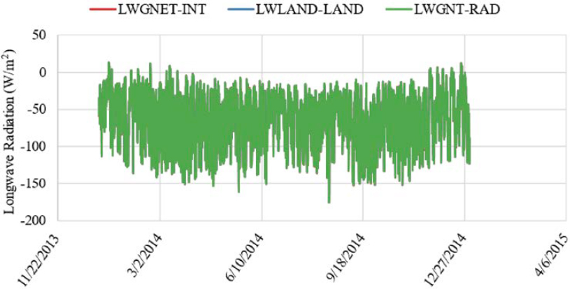
Figure 2 shows that almost no distinct differences existed between the three MERRA-2 data tables for this variable for a 7-day period in July 2014. The location for this example is near Indianapolis, Indiana, where there are no large bodies of water, which explains why there are no
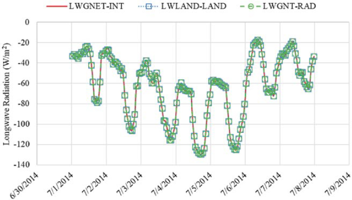
large differences in longwave radiation between the LAND, INT, and RAD MERRA-2 tables. When a particular node and/or grid box includes areas over water, a larger difference is expected. Figure 3 shows the same data for all of 2014, which shows a similar trend as observed for the 7-day period.
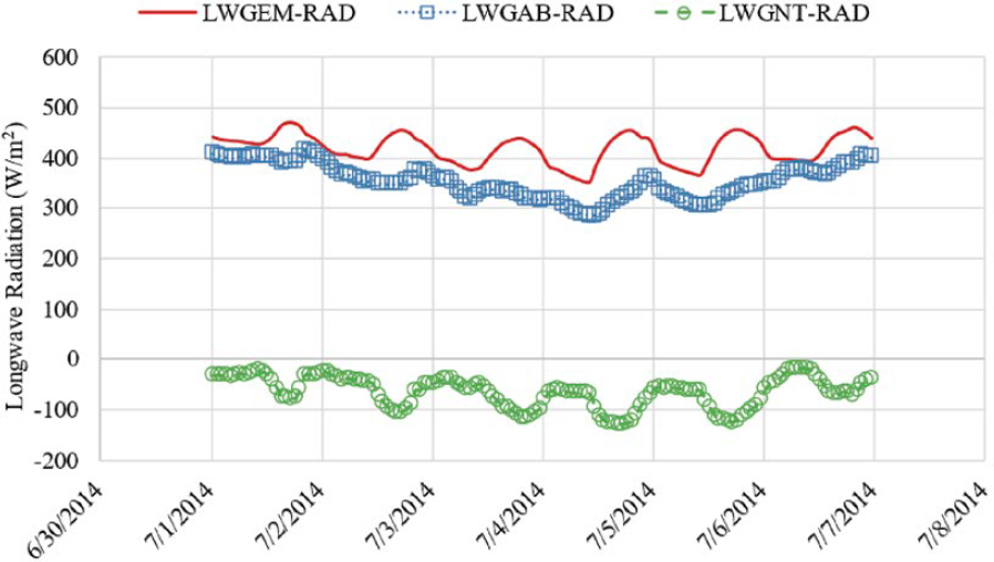
The net incoming (+) and outgoing (−) longwave radiation variables within the RAD MERRA-2 table, which are used to determine the total net longwave radiation for a specific grid point location, are listed here:
- LWGAB-RAD – Surface absorbed longwave radiation over land and water areas within nodal area.
- LWGEM-RAD – Longwave flux emitted from the surface over land and water areas within nodal area.
- LWGNT-RAD – Surface net downward longwave flux over land and water areas within nodal area.
Figure 4 shows an example of each variable for a 7-day period in July 2014. The net downward longwave flux (LWGNT-RAD) represents the difference between the incoming longwave radiation absorbed by the surface (LWGAB-RAD) and the outgoing longwave radiation emitted by the surface (LWGEM-RAD). Typically, the emitted longwave radiation is greater than the absorbed longwave radiation, which results in a net negative value, as observed in Figure 4.
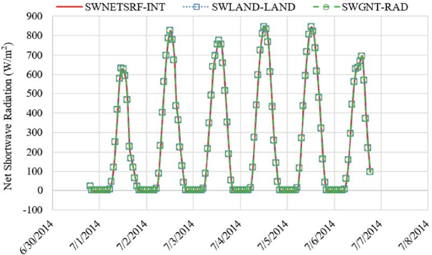
Shortwave Radiation
The net incoming shortwave radiation at the Earth’s surface for the three different MERRA-2 data tables are listed and defined here:
- SWLAND-LAND – Net shortwave radiation over land area only within total nodal area.
- SWNETSRF-INT – Surface net downward shortwave flux over land and water within nodal area.
- SWGNT-RAD – Surface net downward shortwave flux over land and water within nodal area.
Figure 5 illustrates the 7-day hourly net shortwave radiation values from the three MERRA-2 data tables. Minimal differences were observed between the three variables, indicating no significant difference in water fraction within the nodal area.
Total Net Radiation
The total net radiation, which was calculated using the net shortwave and net longwave data presented previously, at the Earth’s surface for the three different MERRA-2 data tables is listed and defined here:
- TOTALNET-LAND = SWLAND-LAND + LWLAND-LAND
- TOTALNET-INT = SWNETSRF-INT + LWGNET-INT
- TOTALNET-RAD = SWGNT-RAD + LWGNT-RAD
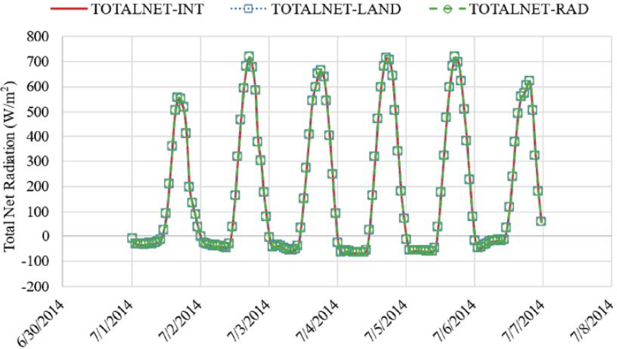
The total net solar radiation for each of the three MERRA-2 data tables is illustrated in Figure 6. For this example, the results are nearly identical between the different data tables, which is expected since the individual components (i.e., shortwave and longwave radiation indices) are also nearly identical. It is expected that larger differences will be observed between the LAND, INT, and RAD datasets when the nodal area includes a larger fraction of water.
Locations with Larger Water Fractions
In areas where the MERRA-2 nodal area has a larger fraction of water, differences will be observed between the three data tables. Typically, the longwave radiation is affected the most because of the differences between how water and land emit the longwave radiation back into the atmosphere. The MERRA-2 LAND data showed lower net longwave radiation compared to the other two datasets, as shown in Figure 7, for a grid point location near Los Angeles, California (CA). Overall, the total net radiation (i.e., shortwave and longwave) did show a slight difference between the different datasets because of the differences in longwave radiation.
3.1.3 Final List of Variables
Based on the comparisons presented in this section, the final list of MERRA-2 variables for different MERRA-2 data collections is summarized in Table 8.
3.1.4 Proposed Process to Extract and Include Input Variables
The following list is a proposed step-by-step process for updating the LTPP InfoPave Climate Tool with additional MERRA-2 variables:
- Update LTPP InfoPave MERRA database design to accommodate additional selected climate data attributes.
- Deploy Amazon Relational Database Service (RDS) database for Oracle to hold the extracted data for the selected climatic data attributes.
- Deploy an application server to host the utility applications for data download and processing.
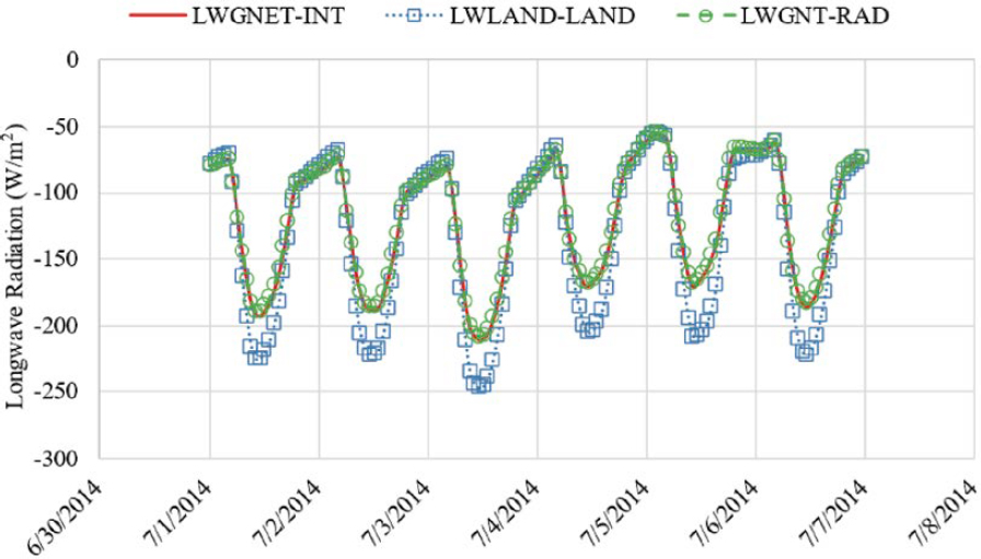
Table 8. MERRA-2 data tables and variables to analyze in depth.
| MERRA-2 Table Name | MERRA-2 Variables | MERRA-2 Variable Description |
| Land surface diagnostics (tavg1_2d_lnd_Nx) | LWLAND | Net longwave over land only |
| SWLAND | Net shortwave over land only | |
| LHLAND | Latent heat flux land | |
| SHLAND | Sensible heat flux land | |
| PRECTOTLAND | Total precipitation land; bias corrected | |
| Vertically integrated diagnostics (tavg1_2d_int_Nx) | LWGNET | Surface net downward longwave flux |
| SWNETSRF | Surface net downward shortwave flux | |
| PRECLS | Large scale rainfall | |
| Radiation diagnostics (tavg1_2d_rad_Nx) | LWGAB | Surface absorbed longwave radiation |
| LWGEM | Longwave flux emitted from surface | |
| LWGNT | Surface net downward longwave flux | |
| LWTUP | Upwelling longwave flux at TOA | |
| SWGDN | Surface incoming shortwave flux | |
| SWGNT | Surface net downward shortwave flux |
- Download MERRA-2 Product raw files for additional selected climate data attributes.
- Extract data from the raw files and populate the temporary database.
- Update the LTPP InfoPave MERRA database schema based on the updated design.
- Move the extracted data to the LTPP InfoPave MERRA database.
- Process the hourly data and populate the summary and roll up tables.
- Develop metadata for the additional climate data attributes.
- Update the LTPP InfoPave Climate Tool to include newly added climate data attributes (optional).
- Update the LTPP InfoPave MERRA Extraction Service to include newly added climate data attributes (optional).
- Back up and decommission the Amazon RDS and application servers.
3.2 Developing Enhancements of Climatic Inputs and Related Models for Future Incorporation in Pavement ME Design
3.2.1 Enhance the EICM Earth–Atmosphere Energy Balance Model
3.2.1.1 Use of MERRA-2 Hourly Shortwave and Longwave Radiation Data
In the previous section, the variables listed in Table 8 from different MERRA-2 tables were extracted for 60+ locations spanning the continental United States, representing the four LTPP defined climatic regions or zones. The locations and climatic zones from which the MERRA-2 data were extracted are shown in Figure 1.
For each of the locations shown in Figure 1, the following steps were performed to analyze and compare the energy balance variables using different MERRA-2 tables and the empirically calculated longwave, shortwave, and total net radiation at the ground surface:
- Calculate the net longwave, shortwave, and total radiation using the empirical formulas currently implemented in the EICM.
- Extract the longwave and shortwave data variables from each MERRA-2 table listed in Table 8.
- Calculate the annual and monthly descriptive statistics for each location and climatic region.
- Compare the calculated net longwave, shortwave, and total radiation based on the empirical formulas (Step 1) to the equivalent MERRA-2 variables.
- Determine whether significant differences exist between the MERRA-2 data variables and the empirically calculated results from the EICM.
The results for each component of the total energy balance equation are summarized in the following section.
Analysis Methods
For each of the climatic variables (i.e., longwave, shortwave, and total net radiation), the following procedure was employed to determine whether statistically significant differences exist between the EICM-calculated energy balance values and the MERRA-2 variables.
Statistical Analysis Definitions and Procedure
- Perform a two-way analysis of variance (ANOVA) to determine whether a significant difference exists in mean values between climate datasets and climate zones using the selected locations.
- – Dependent variable: Mean annual longwave radiation
- – Independent variables:
- Climate dataset with four factor levels (i.e., EICM, LAND, INT, and RAD)
- Climate zone with four factor levels (i.e., wet freeze, wet non-freeze, dry freeze, and dry non-freeze)
-
ANOVA model form:
- – Mean annual value (longwave, shortwave, total net radiation) = climate dataset + climate zone + climate dataset * climate zone
- – Main effects: climate dataset + climate zone
- – Contrasts or interactive terms: climate dataset * climate zone
- Alternative model form:
- – Mean = climate dataset * climate zone
- – This model will test both the main effects and interactive effects.
- If any of the main effects or interactive effects were found to be significant, the Tukey Honest Significant Difference (HSD) test would be performed to determine which levels within each main effect and interactive effects were found to be significant.
Define Hypotheses
- Is there a difference between the climate datasets for longwave, shortwave, and total net radiation?
- – Null Hypothesis: There is no difference between the EICM-calculated values and any of the MERRA-2 datasets.
- – Alternative Hypothesis: There is a difference in one or more of the climate datasets used in the analysis.
- Is there a difference between the climate zones within each climate dataset?
- – Null hypothesis: There is no difference between the climate zones within each climate dataset.
- – Alternate Hypothesis: There is a difference in any of the climate zones.
- Are there any interactive effects between the independent variable groups or within each variable group?
- – Null hypothesis: There is no difference between or within each independent variable group.
- – Alternate Hypothesis: There is a difference between or within any of the independent variable groups.
The analysis results are presented and discussed for each climate variable in the following sections:
- Net Longwave Radiation Analysis Results
- Net Shortwave Radiation Analysis Results
- Net Total Radiation Analysis and Results
Net Longwave Radiation Analysis Results
Results and Discussion. The boxplot distributions of average annual net longwave radiation were generated to compare the range of values included for each climate dataset, as shown in Figure 8. The same data are then separated by each climate region, as shown in Figure 9. Within each figure, the value shown represents the median value, the box represents the interquartile range (IQR), and the whisker lines represent values no higher than 1.5 times above and below the IQR.
The following observations were made:
- The mean annual net longwave radiation is a negative value because the outgoing longwave radiation emitted from the surface is greater than the longwave radiation absorbed from the atmosphere. It is assumed that the incoming longwave radiation is positive while the outgoing or emitted longwave radiation is negative.
- The EICM-calculated net longwave radiation showed similar magnitudes to the MERRA-2 data when all climatic zones are included, as shown in Figure 8. When the data are separated by climatic zone (Figure 9), it can be seen that similar values were observed for the wet-freeze locations while larger differences were observed for the other three climatic zones. The larger
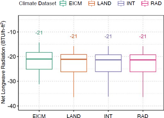
- differences observed for the climatic zones outside of wet-freeze are not surprising because the empirical equations were originally developed using data from locations around the mid-western United States, which is one of the limitations within the EICM addressed in this study.
- The largest overall difference between the EICM-calculated longwave radiation and the MERRA-2 data was observed in the dry freeze and dry non-freeze climatic zones. In both cases, the EICM empirical calculations showed higher net longwave radiation compared to the MERRA-2 data.
The ANOVA statistical analysis results are summarized in Table 9. The highlighted cells in Tables 9 through 14 denote the statistical significance of the independent variables at an alpha level of 0.05. The results show that both main effects (i.e., climate dataset and climate zone) and interactive effects were significantly different than the null hypothesis and conclude that one or
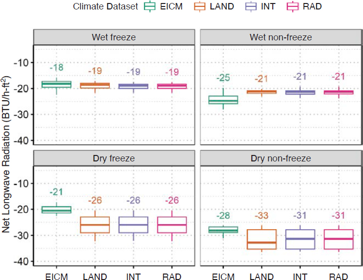
Table 9. ANOVA results for longwave radiation testing main and interactive effects.
| Model Term | Degrees of Freedom (DF) | Sum Sq. | Mean Sq. | Statistic | P-Value |
|---|---|---|---|---|---|
| climate.dataset | 3.000 | 77.100 | 25.700 | 3.499 | 0.016 |
| climate.zone | 3.000 | 3,778.237 | 1,259.412 | 171.459 | 0.000 |
| climate.dataset:climate.zone | 9.000 | 428.215 | 47.579 | 6.478 | 0.000 |
| residuals | 248.000 | 1,821.627 | 7.345 |
more mean differences were found to be different. To identify which groups and levels were significant, the Tukey HSD test was performed to compare multiple comparisons simultaneously.
The results from the Tukey HSD analysis are summarized in Table 10. Adjusted p-values with four asterisks have a significance level equal to 0, p-values with one asterisk have a significance level greater than 0.01 but less than 0.05, and p-values deemed not significant have a significance level greater than 0.05 (these definitions also apply to the adjusted p-values in Tables 12 and 14). The Group 1 variables were compared to the corresponding Group 2 variables to determine whether the means were significantly different from one another. The complete analysis compares all combinations between the climate dataset levels and climate zone levels. Some of these combinations are not necessarily relevant to the overall conclusions and were excluded from Table 10. One such example is the interaction between the EICM dataset within the wet-freeze climate zone compared to the MERRA-2 RAD dataset in the dry-freeze climate zone. A significant difference could be within that combination. Instead, the comparisons were reported when the climate zone from Group 1 was equal to Group 2. Based on the results shown, the following items were highlighted:
- The EICM empirically calculated longwave radiation showed a statistically significant difference when compared to the MERRA-2 INT and RAD tables and not the LAND table.
- None of the MERRA-2 tables showed a statistically significant difference when compared to one another.
- All climatic regions were significantly different from one another.
- The interactive effects found to be significant were the EICM data within the dry-freeze climatic zone compared to the MERRA-2 LAND, INT, and RAD data. These results coincide with the boxplot summaries shown in Figure 9 for the dry freeze climatic zone.
In summary:
- Statistically significant differences were observed between the EICM empirically calculated longwave radiation and the MERRA-2 datasets and between different climatic zones.
- The most important finding from this analysis is that the empirical equations used to calculate longwave radiation showed significant differences in climatic regions, which were not accounted for when the models were developed. Specifically, the differences between the EICM and MERRA-2 data are a function of the following:
- – Constants included in the empirical method were derived from data primarily collected in the Midwestern United States and the wet freeze climatic region. The constants are likely not representative of the other climatic regions.
- – Differences between cloud cover and how it affects the total longwave radiation. The EICM requires a single value for overall cloud cover, while the MERRA-2 data are assimilated based on cloud cover at different heights throughout. The cloud cover height can affect the amount of longwave radiation reflected back to the surface.
- Overall, the authors concluded that the MERRA-2 data are a more representative dataset, which does not rely on regression constants or factors derived based on data within a specific climatic region.
Table 10. Summary of important main and interactive effects for longwave radiation.
| Group 1 | Group 2 | Estimate | Conf. Low | Conf. High | Adj. P-Value | Signif? (ns = not significant) |
|---|---|---|---|---|---|---|
| EICM | Land | –1.187 | –2.407 | 0.034 | 0.060 | ns |
| EICM | Int | –1.274 | –2.494 | –0.054 | 0.037 | * |
| EICM | Rad | –1.275 | –2.495 | –0.055 | 0.037 | * |
| Land | Int | –0.088 | –1.308 | 1.133 | 0.998 | ns |
| Land | Rad | –0.089 | –1.309 | 1.132 | 0.998 | ns |
| Int | Rad | –0.001 | –1.221 | 1.219 | 1.000 | ns |
| Wet freeze | Wet non-freeze | –3.125 | –4.208 | –2.043 | 0.000 | **** |
| Wet freeze | Dry freeze | –5.587 | –6.760 | –4.413 | 0.000 | **** |
| Wet freeze | Dry non-freeze | –11.758 | –13.145 | –10.371 | 0.000 | **** |
| Wet non-freeze | Dry freeze | –2.461 | –3.658 | –1.264 | 0.000 | **** |
| Wet non-freeze | Dry non-freeze | –8.632 | –10.039 | –7.225 | 0.000 | **** |
| Dry freeze | Dry non-freeze | –6.171 | –7.649 | –4.693 | 0.000 | **** |
| EICM:Wet freeze | Land:Wet freeze | –0.383 | –3.212 | 2.446 | 1.000 | ns |
| EICM:Wet freeze | Int:Wet freeze | –0.602 | –3.430 | 2.227 | 1.000 | ns |
| EICM:Wet freeze | Rad:Wet freeze | –0.590 | –3.419 | 2.238 | 1.000 | ns |
| Land:Wet freeze | Int:Wet freeze | –0.218 | –3.047 | 2.610 | 1.000 | ns |
| Land:Wet freeze | Rad:Wet freeze | –0.207 | –3.036 | 2.622 | 1.000 | ns |
| Int:Wet freeze | Rad:Wet freeze | 0.011 | –2.818 | 2.840 | 1.000 | ns |
| EICM:Wet non-freeze | Land:Wet non-freeze | 2.269 | –0.698 | 5.236 | 0.371 | ns |
| EICM:Wet non-freeze | Int:Wet non-freeze | 2.144 | –0.823 | 5.111 | 0.474 | ns |
| EICM:Wet non-freeze | Rad:Wet non-freeze | 2.139 | –0.828 | 5.106 | 0.478 | ns |
| Land:Wet non-freeze | Int:Wet non-freeze | –0.125 | –3.092 | 2.842 | 1.000 | ns |
| Land:Wet non-freeze | Rad:Wet non-freeze | –0.130 | –3.096 | 2.837 | 1.000 | ns |
| Int:Wet non-freeze | Rad:Wet non-freeze | –0.005 | –2.972 | 2.962 | 1.000 | ns |
| EICM:Dry freeze | Land:Dry freeze | –5.549 | –8.975 | –2.123 | 0.000 | **** |
| EICM:Dry freeze | Int:Dry freeze | –5.582 | –9.008 | –2.157 | 0.000 | **** |
| EICM:Dry freeze | Rad:Dry freeze | –5.586 | –9.012 | –2.160 | 0.000 | **** |
| Land:Dry freeze | Int:Dry freeze | –0.034 | –3.459 | 3.392 | 1.000 | ns |
| Land:Dry freeze | Rad:Dry freeze | –0.037 | –3.463 | 3.389 | 1.000 | ns |
| Int:Dry freeze | Rad:Dry freeze | –0.004 | –3.429 | 3.422 | 1.000 | ns |
| EICM:Dry non-freeze | Land:Dry non-freeze | –3.559 | –7.981 | 0.864 | 0.285 | ns |
| EICM:Dry non-freeze | Int:Dry non-freeze | –3.334 | –7.756 | 1.089 | 0.397 | ns |
| EICM:Dry non-freeze | Rad:Dry non-freeze | –3.351 | –7.774 | 1.072 | 0.388 | ns |
| Land:Dry non-freeze | Int:Dry non-freeze | 0.225 | –4.198 | 4.648 | 1.000 | ns |
| Land:Dry non-freeze | Rad:Dry non-freeze | 0.207 | –4.215 | 4.630 | 1.000 | ns |
| Int:Dry non-freeze | Rad:Dry non-freeze | –0.017 | –4.440 | 4.405 | 1.000 | ns |

Net Shortwave Radiation Analysis Results
Results and Discussion. The boxplot summaries for the annual net shortwave radiation for each climate dataset are shown in Figure 10. Figure 11 subdivides the data for each climatic region.
The following observations were made:
- In general, the EICM empirically calculated net shortwave radiation was lower than the MERRA-2 datasets, as shown in Figure 10. The MERRA-2 LAND, INT, and RAD shortwave radiation data were nearly identical.
- When comparing the boxplots for each climate zone, as shown in Figure 11, the EICM-calculated shortwave radiation was less than the MERRA-2 datasets for all climatic zones.
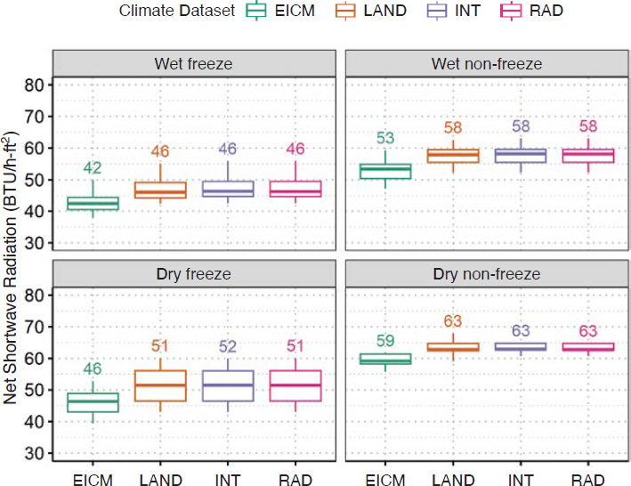
Table 11. ANOVA results for shortwave radiation testing main and interactive effects.
| Model Term | DF | Sum Sq. | Mean Sq. | Statistic | P-Value |
|---|---|---|---|---|---|
| climate.dataset | 3.000 | 1,161.117 | 387.039 | 16.567 | 0.000 |
| climate.zone | 3.000 | 8,287.454 | 2,762.485 | 118.248 | 0.000 |
| climate.dataset:climate.zone | 9.000 | 7.437 | 0.826 | 0.035 | 1.000 |
| residuals | 248.000 | 5,793.716 | 23.362 |
- The wet-freeze and dry non-freeze climatic zones showed the smallest difference between the EICM-calculated and MERRA-2 net shortwave radiation, while the largest differences were observed in the dry freeze and wet non-freeze climate zones.
- For the locations selected, the dry-freeze climate zone showed the largest range of values, as represented by the IQR.
- The differences between the EICM-calculated and MERRA-2 datasets observed for net longwave radiation are most likely due to how cloud cover or percent sunshine is accounted for and the empirical equation constants derived using locations within the wet-freeze climatic region.
The ANOVA statistical analysis results for net shortwave radiation are summarized in Table 11. The results show that only the main effects (i.e., climate dataset and climate zone) were significantly different, while the interaction terms were not. This result indicates that the interaction term can be removed from the ANOVA model. Since the main effects had significantly different means, it was concluded that one or more mean differences were different. The Tukey HSD test was performed to identify which levels within the climate dataset and climate zone are different from one another. Since the interactive effects were not found to be significant, the ANOVA model was updated to only include the main effects.
The results from the Tukey HSD analysis are summarized in Table 12. The Group 1 variables were compared to the corresponding Group 2 variables to identify which combination of levels
Table 12. Summary of important main and interactive effects for shortwave radiation.
| Group 1 | Group 2 | Estimate | Conf. Low | Conf. High | Adj. P-Value | Signif? |
|---|---|---|---|---|---|---|
| EICM | Land | 4.700 | 2.561 | 6.839 | 0.000 | **** |
| EICM | Int | 4.917 | 2.778 | 7.055 | 0.000 | **** |
| EICM | Rad | 4.901 | 2.762 | 7.040 | 0.000 | **** |
| Land | Int | 0.217 | –1.922 | 2.355 | 0.994 | ns |
| Land | Rad | 0.201 | –1.937 | 2.340 | 0.995 | ns |
| Int | Rad | –0.015 | –2.154 | 2.123 | 1.000 | ns |
| Wet freeze | Wet non-freeze | 9.182 | 7.284 | 11.080 | 0.000 | **** |
| Wet freeze | Dry freeze | 3.912 | 1.855 | 5.969 | 0.000 | **** |
| Wet freeze | Dry non-freeze | 16.605 | 14.175 | 19.036 | 0.000 | **** |
| Wet non-freeze | Dry freeze | –5.270 | –7.368 | –3.172 | 0.000 | **** |
| Wet non-freeze | Dry non-freeze | 7.423 | 4.958 | 9.889 | 0.000 | **** |
| Dry freeze | Dry non-freeze | 12.693 | 10.103 | 15.283 | 0.000 | **** |
is significantly different from one another. Based on the results shown, the following observations were highlighted:
- The EICM empirically calculated shortwave radiation showed a statistically significant difference when compared to the any of the MERRA-2 datasets.
- Similar to longwave radiation, none of the MERRA-2 datasets showed a statistically significant difference when compared to another MERRA-2 dataset.
- All climatic regions were significantly different from one another.
In summary:
- For shortwave radiation, the ANOVA results showed that statistically significant differences were found for the main effects (i.e., climate dataset and climate zone). None of the interactive effects resulted in a significant difference and were removed from the ANOVA model.
- The EICM calculated net shortwave radiation was found to be significantly different than all of the MERRA-2 datasets.
- Overall, the authors concluded that the MERRA-2 datasets were more representative for different climate zones compared to the empirically calculated net shortwave radiation.
Net Total Radiation Analysis Results
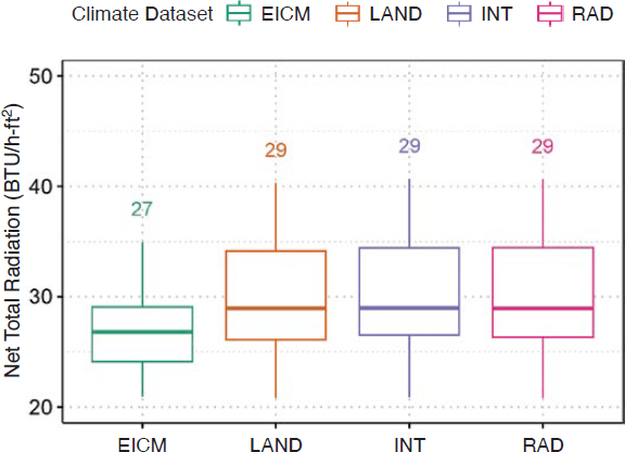
Results and Discussion. The total net radiation is calculated by summing the net shortwave and net longwave radiation. The boxplot summary for total net radiation for each climate dataset is shown in Figure 12, while the same data separated by climate zone are shown in Figure 13.
The following observations were made:
- The total net radiation for the EICM dataset showed a lower median value compared to any of the MERRA-2 datasets. Additionally, the range of values was also much less compared to the MERRA-2 datasets.
- The MERRA-2 datasets showed nearly identical boxplot summaries.
- After separating the climate datasets for each climate zone, as shown in Figure 13, several differences were observed. The EICM total net radiation within the wet freeze and wet non-freeze climate zones was less than the MERRA-2 total net radiation datasets. The EICM-calculated dry freeze and dry non-freeze zones showed median values much closer in magnitude and range compared to the MERRA-2 datasets.
- The differences observed between the total net radiation were similar to those observed and discussed for net shortwave radiation.

The results from the ANOVA for net total radiation are summarized in Table 13. The results show that both the main effects (i.e., climate dataset and climate zone) and interactive effects had significantly different means. The Tukey HSD test was performed to identify which levels within the climate dataset and climate zone were different from one another.
The results from the Tukey HSD analysis are summarized in Table 14. Based on the results, the following observations were documented:
- The EICM empirically calculated total net radiation showed a statistically significant difference compared to all three of the MERRA-2 datasets, while the MERRA-2 datasets were not significantly different from one another.
- All comparisons between levels of climate zones were significantly different except for the comparison between the wet non-freeze and dry non-freeze climate zones.
- Two of the interactive effects resulted in significant differences. The EICM data within the wet freeze and wet non-freeze climatic zones were significantly different than their MERRA-2 counterparts within the same climate zone. None of the dry freeze and dry non-freeze comparisons resulted in significantly different means.
Table 13. ANOVA results for total net radiation testing of main and interactive effects.
| Model Term | DF | Sum Sq. | Mean Sq. | Statistic | P-Value |
|---|---|---|---|---|---|
| climate.dataset | 3.000 | 640.015 | 213.338 | 17.620 | 0.000 |
| climate.zone | 3.000 | 2,766.998 | 922.333 | 76.177 | 0.000 |
| climate.dataset:climate.zone | 9.000 | 384.063 | 42.674 | 3.525 | 0.000 |
| residuals | 248.000 | 3,002.706 | 12.108 |
Table 14. Summary of important main and interactive effects for total net radiation.
| Group 1 | Group 2 | Estimate | Conf. Low | Conf. High | Adj. P-Value | Signif? (ns = not significant) |
|---|---|---|---|---|---|---|
| EICM | Land | 3.513 | 1.947 | 5.080 | 0.000 | **** |
| EICM | Int | 3.642 | 2.076 | 5.209 | 0.000 | **** |
| EICM | Rad | 3.626 | 2.059 | 5.193 | 0.000 | **** |
| Land | Int | 0.129 | – 1.438 | 1.696 | 0.997 | ns |
| Land | Rad | 0.113 | – 1.454 | 1.679 | 0.998 | ns |
| Int | Rad | –0.016 | – 1.583 | 1.550 | 1.000 | ns |
| Wet freeze | Wet non-freeze | 6.057 | 4.666 | 7.447 | 0.000 | **** |
| Wet freeze | Dry freeze | –1.675 | – 3.181 | –0.168 | 0.023 | * |
| Wet freeze | Dry non-freeze | 4.848 | 3.067 | 6.628 | 0.000 | **** |
| Wet non-freeze | Dry freeze | –7.731 | – 9.268 | –6.194 | 0.000 | **** |
| Wet non-freeze | Dry non-freeze | –1.209 | – 3.015 | 0.597 | 0.310 | ns |
| Dry freeze | Dry non-freeze | 6.522 | 4.625 | 8.420 | 0.000 | **** |
| EICM:Wet freeze | Land:Wet freeze | 3.930 | 0.298 | 7.562 | 0.020 | * |
| EICM:Wet freeze | Int:Wet freeze | 4.058 | 0.426 | 7.690 | 0.013 | * |
| EICM:Wet freeze | Rad:Wet freeze | 4.025 | 0.393 | 7.657 | 0.015 | * |
| Land:Wet freeze | Int:Wet freeze | 0.128 | – 3.504 | 3.760 | 1.000 | ns |
| Land:Wet freeze | Rad:Wet freeze | 0.095 | – 3.537 | 3.727 | 1.000 | ns |
| Int:Wet freeze | Rad:Wet freeze | –0.033 | – 3.665 | 3.599 | 1.000 | ns |
| EICM:Wet non-freeze | Land:Wet non-freeze | 7.052 | 3.243 | 10.861 | 0.000 | **** |
| EICM:Wet non-freeze | Int:Wet non-freeze | 7.082 | 3.273 | 10.891 | 0.000 | **** |
| EICM:Wet non-freeze | Rad:Wet non-freeze | 7.068 | 3.259 | 10.877 | 0.000 | **** |
| Land:Wet non-freeze | Int:Wet non-freeze | 0.030 | – 3.779 | 3.839 | 1.000 | ns |
| Land:Wet non-freeze | Rad:Wet non-freeze | 0.016 | –3.793 | 3.825 | 1.000 | ns |
| Int:Wet non-freeze | Rad:Wet non-freeze | –0.014 | –3.823 | 3.795 | 1.000 | ns |
| EICM:Dry freeze | Land:Dry freeze | –0.112 | –4.510 | 4.287 | 1.000 | ns |
| EICM:Dry freeze | Int:Dry freeze | –0.141 | –4.540 | 4.257 | 1.000 | ns |
| EICM:Dry freeze | Rad:Dry freeze | –0.121 | –4.520 | 4.277 | 1.000 | ns |
| Land:Dry freeze | Int:Dry freeze | –0.030 | –4.428 | 4.369 | 1.000 | ns |
| Land:Dry freeze | Rad:Dry freeze | –0.009 | –4.408 | 4.389 | 1.000 | ns |
| Int:Dry freeze | Rad:Dry freeze | 0.020 | –4.378 | 4.419 | 1.000 | ns |
| EICM:Dry non-freeze | Land:Dry non-freeze | 0.673 | –5.006 | 6.351 | 1.000 | ns |
| EICM:Dry non-freeze | Int:Dry non-freeze | 1.288 | –4.391 | 6.966 | 1.000 | ns |
| EICM:Dry non-freeze | Rad:Dry non-freeze | 1.247 | –4.431 | 6.926 | 1.000 | ns |
| Land:Dry non-freeze | Int:Dry non-freeze | 0.615 | –5.063 | 6.293 | 1.000 | ns |
| Land:Dry non-freeze | Rad:Dry non-freeze | 0.574 | –5.104 | 6.253 | 1.000 | ns |
| Int:Dry non-freeze | Rad:Dry non-freeze | –0.041 | –5.719 | 5.638 | 1.000 | ns |
In summary:
- For total net radiation, the ANOVA results showed that statistically significant differences were found for the main effects (i.e., climate dataset, climate zone) and interactive effects.
- The EICM-calculated total net radiation was significantly different than all of the MERRA-2 datasets.
Summary and Conclusions
Based on the results presented, the following conclusions were reported:
- The EICM empirically calculated net longwave, shortwave, and total radiation values were significantly different than the MERRA-2 datasets.
- The MERRA-2 LAND, INT, and RAD tables were not significantly different than one another for net longwave, shortwave, and total radiation. Any of the datasets can be selected to populate hourly shortwave and longwave radiation for use in the EICM. The authors recommend using the MERRA-2 LAND table because it only represents the climatic conditions over land.
- Many of the differences between the EICM-calculated net longwave and shortwave radiation are due to the models and regression constants being developed using data from a specific region, which is not representative of other climatic zones or locations.
- The authors recommend enhancing the EICM by allowing the use of hourly longwave and shortwave radiation instead of the empirical equations currently used.
3.2.1.2 Investigate the Predefined Limits Set on the Convective Heat Transfer Equations
The heat transfer due to convection at the Earth’s surface, Qc, is calculated using the following equation:
Qc = H(Tair − T1)
The convection coefficient, H, is computed using an empirical equation developed by Vehrencamp (3, 14) as shown here:
where Vm is the average of the air temperature and pavement surface temperature in K, Uwind is the wind velocity in mph converted to m/s (1 mph = 0.447 m/s), T1 is the surface temperature in °C, and Tair is the air temperature in °C. The value of 122.93 converts the units from g − cal/min − cm2 − °C to BTU/h − ft2 − °F. The wind velocity input in the EICM is in mph and converted to m/s, hence the 0.447 multiplier in the equation. The value of 1.33 is not well defined and is of an unknown origin. The maximum allowed convection coefficient is a hard-coded value set to 3.0 BTU/h − ft2 − °F. The value was selected to ensure stability within the analysis module when the analysis increments are large. The EICM within the PMED uses an analysis increment of 0.1 h, which is short enough not to cause any stability issues. Therefore, the maximum convection coefficient can be adjusted or removed entirely. The convection coefficient limit value within the EICM input file was adjusted to quantify the impact on the predicted output results. Several values were used; however, none of them had any impact on the predicted outputs.
3.2.2 EICM Feature Enhancements
3.2.2.1 Spatial Interpolation Methods
Currently Implemented Methods
The PMED software allows users to create a “virtual” climate station when their specific project location is too far from a MERRA-2 grid point. The Mechanistic–Empirical Pavement Design Guide: A Manual of Practice (MEPDG MOP) (15) also suggests using a virtual climate station when significant elevation differences are observed between the MERRA-2 grid point location and a selected location. The default search algorithm within the PMED software automatically filters the displayed MERRA-2 grid points by elevation closest to the actual selected location and then by distance. Once multiple MERRA-2 grid point locations are selected, the PMED software creates a virtual climate station using the inverse squared distance weighting method as mentioned in the literature review. For illustration purposes, the PMED software was used to create a virtual station to represent a specific MERRA-2 grid point for two locations. The first location represents a relatively flat area, while the second represents an area with larger elevation differences between MERRA-2 grid points. Figure 14 illustrates the selected grid point locations for the first example, while Figure 15 represents the selected locations for the second example. The green virtual station point locations in Figures 14a and 15a are used to interpolate the data for the green single station point locations in Figures 14b and 15b, respectively. The blue virtual and single station point locations in both figures overall represent the available MERRA-2 gridpoint locations.
The single station and virtual station analysis compares the different hourly climate data that feed into the EICM analysis module. The comparisons consist of air temperature for this analysis. The virtual or interpolated station data are expected to be a reasonable representation of the single station data. Each hourly climate data file has continuous hourly data from 1985 to 2018. The monthly average temperature values are compared for the flat and mountainous locations. Figure 16 illustrates the differences between the two geographical locations for the virtual climate station and the single station. The results show that the monthly average temperatures for the virtual station are almost identical to the single station data for the flat region. Alternatively,


Figure 15. MERRA-2 grid point locations selected to compare a virtual station to an individual MERRA-2 grid point for a highly variable elevation area.
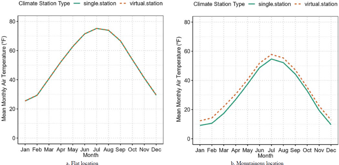
a clear difference is observed between the virtual climate station and single climate station for the mountainous location. For this case, the virtual station consistently showed higher annual temperatures compared to the single station. These differences are not surprising because the hourly MERRA-2 data are grid based and represent a specific elevation, latitude, and longitude. The squared distance weighting algorithm identifies and uses the closest station as the starting point for the interpolation process.
The inverse distance weighted interpolation method may not be appropriate for all geographical locations. Other more sophisticated spatial interpolation methods have been developed that may provide a better estimate for locations between MERRA-2 grid points. Many of these methods were discussed in the literature review. Several of these methods were analyzed to compare differences between interpolated values of temperature, wind speed, precipitation, percent sunshine, and relative humidity to determine whether they provide a better representation for most geographical locations.
Additional Interpolation Methods for Potential Use
The option to create a virtual or “interpolated” climate station or location is significantly important in PMED in the absence of an exact physical weather station near the pavement construction location. The use of additional interpolation methods that can capture the variability between geographical locations, especially elevations or altitude differences, is important to mimic what the pavement structure will experience throughout its life. Using accurate location-specific hourly climate estimates within the EICM will help provide more accurate pavement performance predictions that match the field performance. Several research studies have tested and recommended the use of alternative interpolation methods to overcome some of the identified limitations. A geostatistical interpolation method called kriging was evaluated to determine whether it can provide improved interpolated hourly climate data compared to the inverse distance weighted (IDW) method, especially in areas where large elevation differences over a short distance are present.
Kriging. Spatial interpolation is a fundamental tool in the realm of geostatistics and spatial analysis and essential for estimating values at unsampled locations based on known/provided data points. Among the plethora of interpolation methods available, kriging stands out as a sophisticated and powerful technique with wide-ranging applications across various disciplines, including environmental science, geology, agriculture, and urban planning.
Kriging, initially developed by the French mathematician Georges Matheron in the 1950s, is rooted in the principles of geostatistics and spatial statistics. Unlike simpler interpolation methods, such as IDW or polynomial interpolation, which often lack robustness and fail to account for spatial dependence, kriging offers a more rigorous and statistically sound approach to spatial estimation. The general formula for both interpolators is formed as a weighted sum of the data, which can be calculated using the following equation:
where Z(si) is the measured or known value at the i-th location, λi is a weight factor for the measured value at the i-th location, s0 represents the location where values are interpolated or predicted, and N is the number of measured values.
The weight factor, λi, is based not only on the distance between the measured points and the prediction location but also on the overall spatial arrangement of the measured points. To use the spatial arrangement in the weights, the spatial autocorrelation must be quantified. At its core, kriging leverages the concept of spatial autocorrelation, recognizing that nearby locations tend to
have more similar values than distant ones. By analyzing the spatial structure of the data through variogram modeling, kriging provides not only point estimates but also measures of uncertainty associated with those estimates, making it particularly valuable for decision-making and risk assessment in spatially distributed phenomena. The versatility of kriging lies in its ability to adapt to various spatial patterns and data characteristics. Whether dealing with irregularly spaced point data, continuous surfaces, or categorical variables, kriging offers different variants, such as ordinary, simple, and universal, each tailored to specific scenarios and assumptions.
Variogram. A variogram is a fundamental tool used in geostatistics to characterize the spatial dependence or autocorrelation of a spatial dataset. It quantifies the degree of similarity between pairs of data points as a function of their separation distance. Variograms are particularly important in kriging because they provide information about the spatial structure of the variable being interpolated, which is essential for determining kriging weights and making accurate predictions at unsampled locations. The variogram is calculated by computing the variance of the differences between pairs of data points as a function of their separation distance. The variogram plot typically consists of the distance (lag) on the x-axis and the semi-variance (or variance of differences) on the y-axis. Variograms often exhibit distinct patterns or behaviors, which can be characterized by fitting variogram models. These models help summarize the spatial dependence structure of the data and provide parameters that can be used in kriging interpolation. A subset of the variogram models is discussed briefly here:
- Spherical
- – The spherical model assumes that spatial correlation between data points reaches a maximum value (i.e., sill) at a certain distance (i.e., range), beyond which the correlation levels off and remains constant.
- – The model is characterized by a rapid increase in semi-variance with increasing distance until the range is reached, after which it levels off to the sill value.
- Exponential
- – The exponential model describes spatial correlation as decreasing exponentially with increasing distance between data points.
- – Unlike the spherical model, there is no abrupt leveling-off of the semi-variance; instead, it gradually decreases away from the sill as distance increases.
- Gaussian
- – Similar to the exponential model, the Gaussian model describes spatial correlation as decreasing with increasing distance, but it does so more gradually.
- – The decrease in semi-variance follows a Gaussian or bell-shaped curve, with slower decay compared to the exponential model.
- Hole-Effect
- – The Hole-effect model accounts for situations in which spatial correlation initially decreases at short distances (the “hole” effect), followed by a gradual increase to a plateau.
- – It is often observed in datasets in which localized areas of low correlation surrounded by areas of high correlation are present.
Evaluation of Geographical Distinctions
As discussed earlier, two distinct geographical regions were selected for spatial interpolation: an area with relatively constant elevations (i.e., a flat region) and an area with highly variable elevations changes (i.e., a mountainous region). Each region was represented by a 3-by-3 grid of MERRA-2 data points, where the center grid point is considered the “ground truth” or target value for spatial interpolation. Within each geographical region, the grid points were grouped by similar elevations (lower and higher elevation groups) and another that included all points. This grouping categorization aimed to evaluate the impact of elevation on the interpolation results and assess the performance of kriging across different elevation levels for distinct geographical characteristics.
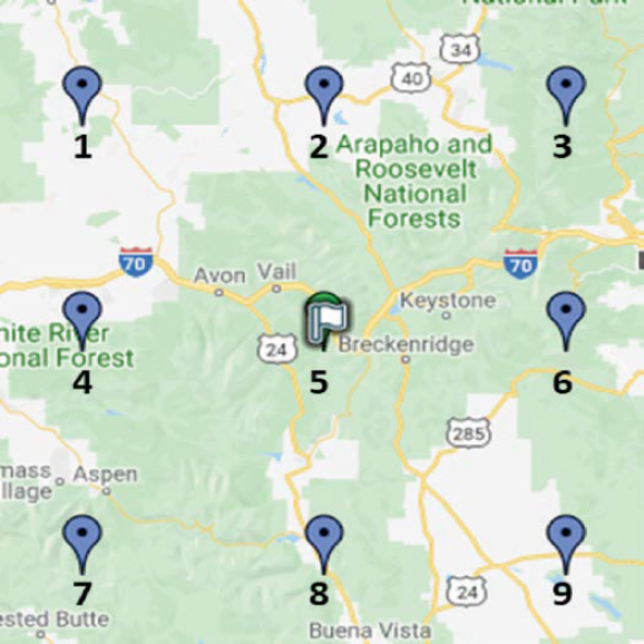
For the mountainous region, the MERRA-2 ID 143543 (Location 5 in Figure 17) was selected along with the surrounding eight MERRA-2 grid points. The eight surrounding points were divided into two groups based on similar elevation levels. Figure 17 illustrates the selected grid point locations for the mountainous region, and Table 15 summarizes the details of each grid point along with their categorization. IDs 1, 2, 4, 8, and 9 in Table 15 were categorized as the low elevation group, while IDs 3, 6, and 7 were categorized as the high elevation group.
Similar to the mountainous region, MERRA-2 ID-144148 (Location 5 in Figure 18), along with the eight surrounding MERRA-2 grid points, was selected to represent the locations with minimal elevation differences for spatial interpolation. Figure 18 illustrates the selected grid
Table 15. Mountainous location summary data.
| ID | MERRA -2 ID | Elevation (ft) | Latitude | Longitude | Elevation Group |
|---|---|---|---|---|---|
| 1 | 144118 | 8,875 | 40.0 | –106.875 | Group 1 |
| 2 | 144119 | 8,095 | 40.0 | –106.250 | Group 1 |
| 3 | 144120 | 11,525 | 40.0 | –105.625 | Group 2 |
| 4 | 143542 | 8,150 | 39.5 | –106.875 | Group 1 |
| 5 | 143543 | 11,270 | 39.5 | –106.250 | Baseline |
| 6 | 143544 | 12,500 | 39.5 | –105.625 | Group 2 |
| 7 | 142966 | 12,811 | 39.0 | –106.875 | Group 2 |
| 8 | 142967 | 9,462 | 39.0 | –106.250 | Group 1 |
| 9 | 142968 | 8,905 | 39.0 | –105.625 | Group 1 |

point locations for the flat region, and Table 16 summarizes the details of each grid point along with the elevation group categories. IDs 1, 2, 3, and 4 in Table 16 were grouped to represent the low elevation group, while IDs 6, 7, 8, and 9 represent the high elevation group.
Spatial Interpolation Results. The data period of each grid point is from 1985 to 2021 and collected temperature, wind speed, percent sunshine, precipitation, and relative humidity for every hour.
As discussed earlier, the grid points at each region were placed into three categories: low elevation points (Group 1), high elevation points (Group 2), and all points (8 points). Spatial interpolation using 2D kriging was then conducted on each category. Moreover, selecting the
Table 16. Flat location summary data.
| ID | MERRA -2 ID | Elevation (ft) | Latitude | Longitude | Elevation Group |
|---|---|---|---|---|---|
| 1 | 144723 | 842 | 40.5 | –88.750 | Group 1 |
| 2 | 144724 | 770 | 40.5 | –88.125 | Group 1 |
| 3 | 144725 | 725 | 40.5 | –87.500 | Group 1 |
| 4 | 144147 | 682 | 40.0 | –88.750 | Group 1 |
| 5 | 144148 | 682 | 40.0 | –88.125 | Baseline |
| 6 | 144149 | 524 | 40.0 | –87.500 | Group 2 |
| 7 | 143571 | 688 | 39.5 | –88.750 | Group 2 |
| 8 | 143572 | 675 | 39.5 | –88.125 | Group 2 |
| 9 | 143573 | 596 | 39.5 | –87.500 | Group 2 |
most appropriate variogram model is crucial for accurate interpolation results. Since variogram modeling involves fitting a theoretical model to empirical variogram data, testing multiple variogram models helps identify the model that best describes the observed spatial dependence patterns. Root mean squared error (RMSE) was used to evaluate model performance and select the most appropriate variogram model for interpolation.
The spatial interpolation results using 2D kriging for a mountainous region are summarized in Table 17. Based on the analysis results, similar RMSE values were exhibited across variogram models within each category. However, considering the consistent pattern across all three categories, where the Gaussian model generally yields the lowest RMSE values for most variables, both Group 1 (low elevation) and Group 2 (high elevation) categories showed similar patterns of performance, with the Gaussian variogram model consistently outperforming other models. However, since the 8-points category exhibited relatively lower RMSE values overall, representing the spatial interpolation using the surrounding eight grid points can capture spatial dependence patterns and produce accurate predictions across variables without considering elevation differences.
The spatial interpolation results using 2D kriging for the relatively flat regions are summarized in Table 18. Based on the analysis results, the 8-points category represents the overall spatial variability across the flat region, without considering elevation differences. The lower RMSE values in this category suggest that the spatial dependence patterns for the variables tend to be more consistent or predictable across different locations in the flat region.
Despite similar RMSE values across variogram models within each category, the Hole-effect variogram model showed the lowest RMSE across the grouping categories and climatic variables overall. Moreover, the higher RMSE for percent sunshine may be influenced by its unique characteristics as a percentage variable or because of localized variability with respect to cloud cover. Standard variogram models might not be able to capture the nonlinearity or high variability associated with the percent sunshine values.
Table 17. Spatial interpolation results using 2D kriging for a mountainous region.
| Interpolation Group | Variogram Model | Temperature (°C) | Wind Speed (mph) | Percent Sunshine (%) | Precipitation (in) | Relative Humidity (%) |
|---|---|---|---|---|---|---|
| 8 Points | Exponential | 5.165 | 2.205 | 11.433 | 0.009 | 8.684 |
| Gaussian | 4.857 | 1.958 | 11.963 | 0.009 | 8.079 | |
| Hole-Effect | 5.681 | 2.134 | 11.841 | 0.010 | 9.432 | |
| Spherical | 5.609 | 2.138 | 11.793 | 0.010 | 9.299 | |
| Group 1 (Low Elevation) | Exponential | 5.664 | 2.559 | 12.736 | 0.011 | 9.183 |
| Gaussian | 4.872 | 2.464 | 12.369 | 0.010 | 8.215 | |
| Hole-Effect | 6.126 | 2.403 | 13.209 | 0.011 | 9.883 | |
| Spherical | 6.099 | 2.415 | 13.158 | 0.011 | 9.788 | |
| Group 2 (High Elevation) | Exponential | 4.830 | 1.760 | 12.597 | 0.010 | 9.356 |
| Gaussian | 4.356 | 1.665 | 12.595 | 0.010 | 8.946 | |
| Hole-Effect | 4.531 | 1.688 | 12.736 | 0.010 | 8.576 | |
| Spherical | 5.145 | 1.815 | 12.777 | 0.010 | 9.792 |
Table 18. Spatial interpolation results using 2D kriging for a flat region.
| Interpolation Group | Variogram Model | Temperature (°C) | Wind Speed (mph) | Percent Sunshine (%) | Precipitation (in) | Relative Humidity (%) |
|---|---|---|---|---|---|---|
| 8 Points | Exponential | 1.089 | 0.963 | 10.962 | 0.017 | 2.810 |
| Gaussian | 1.495 | 1.116 | 13.606 | 0.019 | 3.663 | |
| Hole-Effect | 1.032 | 0.941 | 10.576 | 0.017 | 2.684 | |
| Spherical | 1.048 | 0.946 | 10.674 | 0.017 | 2.723 | |
| Group 1 (Low Elevation) | Exponential | 1.449 | 1.132 | 12.449 | 0.019 | 3.231 |
| Gaussian | 1.556 | 1.166 | 13.053 | 0.019 | 3.499 | |
| Hole-Effect | 1.422 | 1.129 | 12.323 | 0.019 | 3.159 | |
| Spherical | 1.422 | 1.129 | 12.329 | 0.019 | 3.168 | |
| Group 2 (High Elevation) | Exponential | 1.760 | 1.242 | 14.755 | 0.020 | 3.858 |
| Gaussian | 1.771 | 1.249 | 14.857 | 0.021 | 3.886 | |
| Hole-Effect | 1.791 | 1.258 | 14.920 | 0.021 | 3.929 | |
| Spherical | 1.786 | 1.255 | 14.908 | 0.021 | 3.922 |
2D kriging primarily focuses on interpolating values within a 2D plane or surface, such as a map or geographic area. While 2D kriging can capture some aspects of elevation differences within this plane, it does not directly model or interpolate variations in elevation in the vertical dimension. To capture vertical elevation differences directly, 3D kriging was also employed for spatial interpolation to capture spatial variability across both horizontal and vertical dimensions. However, since 3D kriging involves estimating values at unsampled locations within a 3D volume, it requires much more processing time compared to 2D kriging. Therefore, 1 year of data (1985) was utilized for 3D spatial interpolation using the Gaussian and Hole-effect variogram models for the mountainous and flat regions, respectively. This approach was applied separately to each region to generate the interpolated datasets. Table 19 summarizes the 2D and 3D spatial interpolation results for both regions. It should be noted that the results presented in Table 19 for 2D interpolation are based on data from the same period, specifically the year of 1985.
In the mountainous region, 3D interpolation yielded higher RMSE values compared to 2D interpolation across all variables in all categories. Conversely, in the flat region, those two interpolation results showed similar performances; however, 3D interpolation exhibited better performance in Group 1, providing lower RMSE values compared to 2D interpolation for most variables.
The results presented between 2D and 3D kriging were surprising because the initial assumption was that 3D kriging would result in lower RMSE values compared to the 2D analysis since it directly accounts for altitude when calculating the distance between the target location and the other grid points in the analysis. One of the suspected reasons higher RMSE values for 3D kriging were observed was the limited number of locations (i.e., 8 points) selected for this analysis and the highly variable elevation values corresponding to each grid point location.
As an additional check, the baseline grid point location (i.e., Location 5 in Figure 17) was included in the interpolation scheme as an additional point for the kriging interpolation. The location was added to the interpolation scheme because the aim was to study whether the interpolation method can estimate the MERRA-2 values better than when it is not included in the
Table 19. Spatial interpolation results using 2D and 3D kriging for a flat and mountainous regions.
| Geography Type | Interpolation Type | Interpolation Group | Temperature (ºC) | Wind Speed (mph) | Percent Sunshine (%) | Precipitation (in) | Relative Humidity (%) |
|---|---|---|---|---|---|---|---|
| Flat | 3D | 8 Points | 1.193 | 1.026 | 10.824 | 0.015 | 2.423 |
| Group 1 – (Low Elevation) | 1.506 | 1.170 | 12.527 | 0.018 | 2.817 | ||
| Group 2 – (High Elevation) | 2.027 | 1.274 | 15.199 | 0.017 | 3.143 | ||
| 2D | 8 Points | 1.102 | 0.947 | 10.863 | 0.015 | 2.477 | |
| Group 1 – (Low Elevation) | 1.844 | 1.180 | 13.010 | 0.018 | 3.226 | ||
| Group 2 – (High Elevation) | 2.168 | 1.259 | 15.213 | 0.018 | 3.538 | ||
| Mountainous | 3D | 8 Points | 5.388 | 2.306 | 54.682 | 0.042 | 14.526 |
| Group 1 – (Low Elevation) | 5.679 | 2.579 | 24.331 | 0.012 | 8.801 | ||
| Group 2 – (High Elevation) | 5.716 | 1.987 | 13.002 | 0.009 | 9.444 | ||
| 2D | 8 Points | 4.661 | 2.035 | 12.294 | 0.009 | 7.376 | |
| Group 1 – (Low Elevation) | 4.728 | 2.580 | 12.434 | 0.010 | 7.498 | ||
| Group 2 – (High Elevation) | 4.507 | 1.657 | 12.375 | 0.009 | 8.240 |
interpolation dataset. The hypothesized result is lower RMSE value(s) when the baseline grid point is included in the analysis compared to when it is excluded from the analysis.
The following steps were followed to perform additional analysis:
- Add Location 5 to the interpolation dataset to perform kriging with all nine hourly data points.
- Interpolate the hourly climate data at a location close to the MERRA-2 grid point location.
- Adjust the “OrdinaryKriging” function inputs as follows:
- – Adjust the “weight” option to True. This option sets a greater weight for grid points closer to the interpolation location. In this case, Location 5 will be weighted more heavily since it is the closest MERRA-2 grid point to the specified location.
- Additional Use Cases
- – One benefit of the spatiotemporal interpolation methods is that they can interpolate values at multiple points. For example, if multiple coordinates along a roadway are specified, point value estimates can be determined for each point to represent “roadway specific” climate data. The MERRA-2 gridded system could be used to create a network of roadway-specific assimilated climate data.
The analysis results are summarized in Table 20, which showed significantly reduced RMSE values compared to the analysis that used only 8 points. When using the weighted by distance setting, the RMSE reduced further and is more aligned with the RMSE values obtained for the flat regions.
Summary of Results and Recommendations
- The currently implemented IDW interpolation method is adequate for most locations where large elevation changes over short distances are not present.
- Kriging can be more accurate if enough point locations are available and distances are not too large. Additionally, including the weighted setting within the kriging interpolation scheme reduced the overall RMSE.
- Correcting for elevation is still recommended.
- – The 3.5° temperature difference for 1,000 ft of elevation change is appropriate for temperature corrections. It is the standard lapse rate, which is used for aviation purposes. The standard lapse rate is 6.5 °C per km or 3.56 °F per 1,000 ft. The lapse rate is applicable between sea level and 11 km above the Earth’s surface.
- Future considerations
- – Identify points along interstate, state, and county roadways and interpolate hourly climate data based on the roadway network.
- – Integrate the kriging method as an option within the AASHTOWare Pavement ME Design software.
- Open-source Python, R, C#, or other packages may exist that can be integrated to perform the interpolation.
3.2.2.2 Adjusting Constant Deep Ground Temperature
The EICM procedure considers the MAAT as the lower boundary temperature. The current algorithm can be adjusted to set this temperature just above freezing (32 °F/0 °C) in all cases to allow the EICM to run for the areas where the MAAT is usually less than freezing. As a part of the annual updates, the PMED software and EICM, specifically, were updated to account for locations where the MAAT is below freezing. The implemented procedure sets the initial pavement temperature to 55 °F or 12.8 °C, which corresponds to the original value used when the EICM was developed.
Another potential solution for an initial nodal temperature is to use the average temperature corresponding to the unbound or granular base construction month. This solution assumes that the monthly average air temperature is greater than freezing. In most cases, the pavement construction seasons do not start until after the ground has thawed.
3.2.2.3 Investigate Methods to Improve Pavement Temperature Predictions During Precipitation Events
The EICM does not currently directly account for the change in pavement temperature with respect to precipitation. The pavement temperature is expected to closely reflect the air temperature during precipitation events, as the amount of rain or snow will either cool or warm the
Table 20. Spatial interpolation RMSE results using 2D kriging for a mountainous region using nine MERRA-2 grid point locations.
| Comparison Name | Distance Weighted? | Temperature (ºC) | Wind Speed (mph) | Percent Sunshine (%) | Precipitation (in) | Relative Humidity (%) |
|---|---|---|---|---|---|---|
| Original with 8 Points | No | 2.3659 | 0.94691 | 4.3865 | 0.0032533 | 3.4870 |
| Weighted by Distance | Yes | 1.5135 | 0.79046 | 4.3423 | 0.0031488 | 2.9273 |
pavement surface depending on the current climatic conditions. Different methods were investigated to identify potential improvements to the prediction of pavement temperature during precipitation events to closely reflect the measured pavement temperatures.
The following list summarizes the process used to complete this investigation:
- Identify variables within the MERRA-2 LAND database related to precipitation that affect the overall energy balance results. The following variables were identified:
- – Latent Heat Flux
- Defined as LHLAND in MERRA-2.
- Represents the transfer of latent heat between the land surface and the atmosphere due to evaporation and transpiration. It is associated with water vapor. Latent heat plays an important role in the overall water cycle and affects soil moisture and regional climates. Positive values indicate moisture release from the surface to the atmosphere, while negative values indicate moisture update by the surface.
- – Sensible Heat Flux
- Defined as SHLAND in MERRA-2.
- Represents the transfer of sensible heat (i.e., thermal energy) between the land surface and the atmosphere due to temperature differences. It quantifies the heat exchange resulting from the temperature gradient between the land surface and the air just above it. Sensible heat affects local weather patterns, air temperature, and boundary layer dynamics. Positive values indicate heat transfer from the surface to the atmosphere (e.g., warm ground heating the air), while negative values indicate heat transfer from the atmosphere to the surface (e.g., cooling of the ground).
- – Ground Heat Flux
- Defined as GHLAND in MERRA-2.
- Represents the heat transfer between the Earth’s surface (i.e., land) and the atmosphere due to conduction. It quantifies the energy exchange at the land surface. Ground heat flux is crucial for understanding land–atmosphere interactions, which influence local climate, soil temperature, and other non–pavement-related factors, such as vegetation growth. Positive values indicate heat transfer from the ground to the atmosphere (e.g., during daytime), while negative values indicate heat transfer from the atmosphere to the ground (e.g., during nighttime).
- – Total Precipitation
- Defined as PRECTOTLAND in MERRA-2.
- Represents the observation-corrected precipitation rate for specific time increment, 1 h, in this analysis. The raw values are converted from kg m−2 s−1 to mm/h (multiplying by 3,600 s) and then converted to in/h (multiplying by 25.4).
- – Latent Heat Flux
- Compare different energy balance variables to precipitation and identify whether any significant correlations exist.
- Compare different combinations of energy balance variables to calculate the total energy balance (Qrad).
Compare Different Energy Balance Variables
In addition to the variables defined above, additional variables were calculated to combine the radiation data and the heat flux data. The following variables were calculated:
- NetRad: Total net radiation equal to the sum of net shortwave and longwave radiation. These represent the radiative forcing variables.
- NetHeat: Total heat flux equal to the sum of the latent heat flux, sensible heat flux, and ground heat flux.
- TotalBudgetBalance: Total energy budget balance between NetRad and NetHeat. The sum of these two variables should be close to 0.
Figure 19 shows an example of the time series data for the energy variables defined above for a 4-day period in May 2011. The following observations were made:
- NetRad and NetHeat are nearly identical.
- TotalBudgetBalance is about equal to 0 for the selected time period.
- LHLAND, GHLAND, and SHLAND follow similar trends in which the values are much higher during daytime hours compared to nighttime hours.
- Based on these results, the sum of longwave and shortwave radiation is approximately equal to the sum of latent heat flux, sensible heat flux, and ground heat flux.
Compare Different Energy Balance Variables to Precipitation and Identify Whether Any Significant Correlations Exist
The hourly data for an entire year (2013) were extracted and analyzed to identify whether any of the variables defined previously were correlated with one another. Figure 20 shows the scatter-plot matrix comparing each variable in the dataset. Values with three asterisks have a significance level less than 0.001, values with one asterisk have a significance level less than 0.05 but greater than 0.01, and values with no asterisks have a significance level greater than 0.1. The asterisks indicate whether the pairwise comparisons are statistically different than one another. The correlation coefficient, and whether it was found to be statistically significant, is also shown. For the 2013 data subset, precipitation did not show very high correlation coefficients when compared to the other variables. Most of the correlations were significantly different than a correlation coefficient equal to 0. The largest correlation coefficient for precipitation versus other variables was identified for longwave radiation, with a value of 0.235. Much stronger correlations were observed for other variable combinations, such as a value of 0.897 for the latent heat and shortwave radiation comparison. Based on this dataset, precipitation does not show a clear relationship between any of the energy balance parameters. The effects of precipitation on the
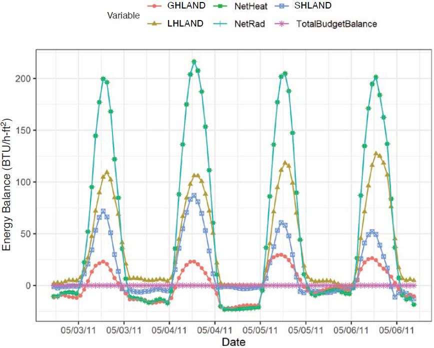
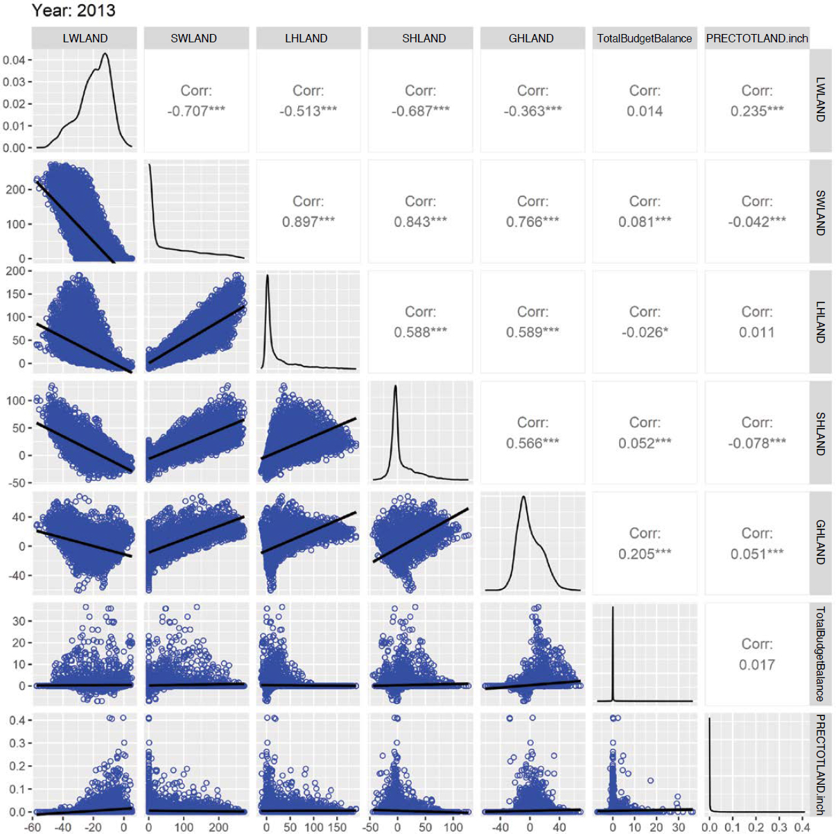
overall energy balance were unclear in this case and were likely accounted for in the latent heat variable or quite small compared to the magnitude of the other variables.
Results and Discussions
The instantaneous effect of precipitation on the pavement temperature is not really shown in the data. One potential reason for this observation is that the impact of precipitation on the surface or skin temperature is accounted for in the latent heat flux variable due to the evaporation and transpiration processes. The effect may also be minimized due to the sensible
heat flux, which is the energy transferred as heat from the Earth’s surface to the atmosphere due to temperature differences. Sensible heat flux includes the conduction and convection processes.
- Assimilated datasets, such as MERRA-2, may not compare well to point-specific measured values due to the modeling process.
- Assimilated datasets follow general trends based on many different sources and cannot capture every situation.
- A direct relationship between precipitation and the energy balance variables, which are used to predict pavement temperature in the EICM, was not found. It is hypothesized that the assimilation process masks some of the effects that may occur for a specific location.
3.3 Validating New or Enhanced Models
The results and findings from the previous tasks were used to validate the results and determine whether the new features provide a better result compared to the original model. The validation procedure consists of several hypothesis tests to determine model adequacy. The two main tests for adequacy include the pairwise comparison between two datasets and a linear regression test on slope and intercept. In addition to the hypothesis test, the RMSE and mean residual error (MRE) are also performed. The validation tests were performed using a subset of LTPP Seasonal Monitoring Program (SMP) pavement test sections from Arizona, Manitoba, Georgia, and New Jersey. The measured and predicted pavement temperatures were compared in the validation process.
3.3.1 Validation Procedure
The validation process used for each SMP site follows the following outline:
- Plot one-to-one comparison between measured and predicted pavement temperature.
- Calculate residual error between measured and predicted pavement temperature and generate a histogram of the residual error using a bin size of 2 °F.
- Perform linear regression to determine the slope and intercept coefficients as well as R2 and goodness of fit hypothesis test results.
- Calculate the RMSE, R2, and MRE and compare the values between measured and predicted pavement temperature.
- Compare the RMSE, R2, and MRE.
3.3.2 Validation Results
The validation results for the Arizona, Manitoba, Georgia, and New Jersey SMP sites are summarized in the following sections. The first surface layer sensor was used for the analysis.
3.3.2.1 Arizona SMP Flexible
One-to-One Comparison
The MERRA-2 shortwave and longwave radiation data were used to calculate the total net radiation, which is used to predict pavement temperature in the EICM. Figures 21 and 22 show the one-to-one comparison between the predicted pavement temperature (y-axis) and measured pavement temperature (x-axis) for the MERRA-2 and PMED methods, respectively. Overall, both figures show a linear trend along the line of equality. The scatter around the line of equality is also similar for both cases, which indicates that the pavement temperature predictions generally

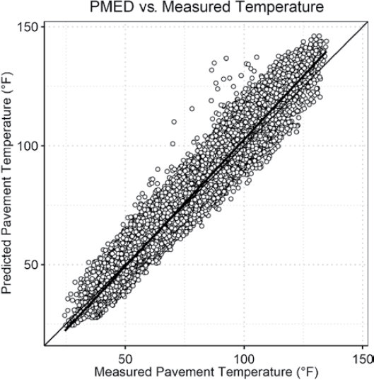
compare well to the measured pavement temperatures. Based on the figures, it is difficult to determine whether the MERRA-2 data resulted in a better fit compared to the empirical model within the EICM.
As an additional comparison, the MERRA-2-predicted pavement temperatures are plotted against the PMED-predicted pavement temperatures, as shown in Figure 23. The comparison shows a linear trend along the line of equality with lower scatter at lower temperatures compared to higher temperatures.
Residual Error Histogram
The residual error between the measured pavement temperature and MERRA-2- and EICM-predicted pavement temperatures were compared to identify which method was best. The residual error was calculated for each hour the measured data were available. The residual error values were grouped into bin categories of approximately 2°. The number of bins depends on the overall range of values included in the dataset. The number of observations within each group was counted as shown in Figure 24. The results show a slight negative bias, as the largest number of residual error observations fell between the −2° through −8° bin categories. Ideally, the majority of observations should fall near the 0° category, but this expectation is not always the case.
Linear Regression and Hypothesis Test Results
The pairwise comparison, intercept, and slope hypothesis test results for the MERRA-2 and EICM/PMED comparisons with the measured pavement temperature data are summarized in Tables 21 and 22, respectively. The mean difference between the predicted and measured pavement temperature was less than 1 for both cases. The MERRA-2 case had a lower mean difference compared to the EICM/PMED dataset. The slope estimates were practically equal to 1, while the intercept values were both negative and less than 5°. The null hypotheses were rejected, which means that the mean difference was statistically significantly different
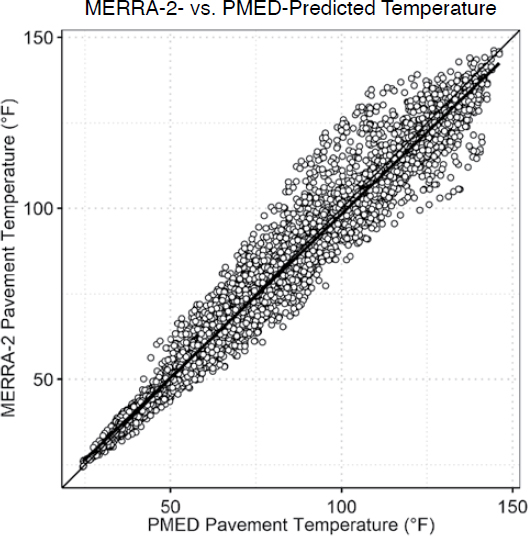

than 0, the intercept was statistically different than 0, and the slope was statistically different than 1. The large number of data points within the dataset is one of the reasons why the null hypotheses were rejected. Practically, these results are similar and both cases compared well to the measured pavement temperatures. The pavement temperatures predicted using the MERRA-2 shortwave and longwave radiation data resulted in a slightly better prediction overall for the Arizona SMP location.
Table 21. MERRA-2 versus measured pavement temperature hypothesis test results for the Arizona SMP site.
| Hypothesis Test | Value Estimate | P-Value |
|---|---|---|
| Paired t-test (mean difference) | –0.3088 | 0.0001 |
| Intercept = 0 | –3.0619 | 0.0000 |
| Slope = 1 | 1.0447 | 0.0000 |
Table 22. PMED-predicted pavement temperature versus measured pavement temperature hypothesis test results for the Arizona SMP site.
| Hypothesis Test | Value Estimate | P-Value |
|---|---|---|
| Paired t-test (mean difference) | –0.9614 | 0.0000 |
| Intercept = 0 | –4.0629 | 0.0000 |
| Slope = 1 | 1.0666 | 0.0000 |
Table 23. MERRA-2-predicted pavement temperature versus PMED-predicted pavement temperature hypothesis test results for the Arizona SMP site.
| Hypothesis Test | Value Estimate | P-Value |
|---|---|---|
| Paired t-test (mean difference) | 0.6527 | 0.0000 |
| Intercept = 0 | 2.6647 | 0.0000 |
| Slope = 1 | 0.9566 | 0.0000 |
The MERRA-2- versus PMED-predicted pavement temperatures were also subjected to the set of hypothesis tests to determine whether statistically or practically significant differences exist between the datasets. The hypothesis test results are summarized in Table 23. The average pairwise difference between the MERRA-2- and PMED-predicted pavement temperatures was less than 1 °F, which is practically insignificant even though the null hypothesis was rejected. The slope and intercept hypothesis tests were also significantly different statistically, while the value estimates were practically the same as the null hypothesis.
RMSE, R2, and MRE
The results presented previously still do not clearly indicate whether the MERRA-2 data resulted in a better prediction compared to the empirical PMED equation. The results were subdivided to calculate the RMSE, R2, and MRE for each month the data were available. Table 24 summarizes the RMSE results for the Arizona SMP site for each month. Overall, the MERRA-2 dataset resulted in a lower RMSE for the majority of months, especially during the summer and fall seasons. Table 25 shows the R2 calculated for each month, which showed a similar trend as the RMSE results. Overall, the MERRA-2 data showed a slightly better prediction compared to the empirical calculations within the EICM and PMED. Table 26 summarizes the MRE for each
Table 24. Monthly RMSE for the Arizona SMP site.
| Month | MERRA-2 vs. Measured | PMED vs. Measured |
|---|---|---|
| Jan | 6.0355 | 6.1559 |
| Feb | 6.4493 | 5.9414 |
| Mar | 7.1083 | 6.7221 |
| Apr | 7.4344 | 7.3978 |
| May | 7.7883 | 8.5479 |
| Jun | 8.3360 | 9.0328 |
| Jul | 9.8134 | 10.3955 |
| Aug | 7.9293 | 9.9765 |
| Sep | 7.7040 | 9.9964 |
| Oct | 6.4802 | 7.8294 |
| Nov | 5.2046 | 7.3840 |
| Dec | 4.9375 | 5.5694 |
Table 25. Monthly R2 for the Arizona SMP site.
| Month | MERRA-2 vs. Measured | PMED vs. Measured |
|---|---|---|
| Jan | 0.77752 | 0.74386 |
| Feb | 0.84323 | 0.84827 |
| Mar | 0.87226 | 0.85098 |
| Apr | 0.87540 | 0.85027 |
| May | 0.89056 | 0.85320 |
| Jun | 0.86343 | 0.85895 |
| Jul | 0.74766 | 0.76337 |
| Aug | 0.83930 | 0.81249 |
| Sep | 0.80248 | 0.78673 |
| Oct | 0.83591 | 0.80521 |
| Nov | 0.84942 | 0.81158 |
| Dec | 0.79310 | 0.79782 |
month. The MRE provides additional information regarding the over- or under-prediction of the pavement temperature compared to the measured values. The MRE is calculated by averaging the difference between the predicted pavement temperature and the measured pavement temperature. A negative value means that the predicted pavement temperature is higher than the measured values. The results show that the MERRA-2 data showed lower MRE values compared to the PMED-predicted temperatures. All of the MERRA-2 monthly MRE values were between −2° and 2°.
Table 26. Monthly MRE for the Arizona SMP site.
| Month | MERRA-2 vs. Measured | PMED vs. Measured |
|---|---|---|
| Jan | 1.50518 | 2.372705 |
| Feb | –1.82726 | –1.147141 |
| Mar | –1.46418 | 0.029663 |
| Apr | –0.79029 | 0.517790 |
| May | 1.29978 | 1.344144 |
| Jun | 1.18647 | –0.103573 |
| Jul | –2.50553 | –3.280188 |
| Aug | –1.03196 | –3.106282 |
| Sep | 0.09553 | –2.663500 |
| Oct | 0.28706 | –1.687261 |
| Nov | –0.75374 | –3.111421 |
| Dec | 0.19611 | –0.758132 |
Overall, the predicted pavement temperatures using the MERRA-2 data were better than the empirical equations included in the EICM/PMED for the Arizona SMP site when compared to the measured pavement temperature.
3.3.2.2 Manitoba SMP Rigid
One-to-One Comparison
The Manitoba LTPP SMP section was selected to compare the predicted and measured pavement temperatures for a colder climate. Figures 25 and 26 show the one-to-one comparison between the predicted pavement temperature and measured pavement temperature for the MERRA-2 and EICM/PMED methods, respectively. Overall, both figures show a linear trend along the line of equality. The scatter around the line of equality is similar for both comparisons and show less scatter at colder pavement temperatures compared to warmer pavement temperatures. The MERRA-2 case resulted in higher pavement temperature predictions compared to the measured values when the overall temperature was higher than 60 °F. Based on the figures, the method included in the EICM/PMED compares slightly better than the MERRA-2-calculated values.
The MERRA-2-predicted pavement temperatures are plotted against the PMED-predicted pavement temperatures, as shown in Figure 27. The comparison shows a linear trend along the line of equality with much less scatter at lower temperatures compared to higher temperatures. In general, good agreement exists between the MERRA-2- and PMED-predicted pavement temperatures.
Residual Error Histogram
The residual error between the measured pavement temperature and the MERRA-2- and EICM-predicted pavement temperatures was compared to identify whether one method is better than the other. The number of observations within each residual error group was counted and summarized using a histogram, as shown in Figure 28. The results show a slight positive bias
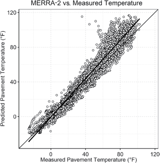
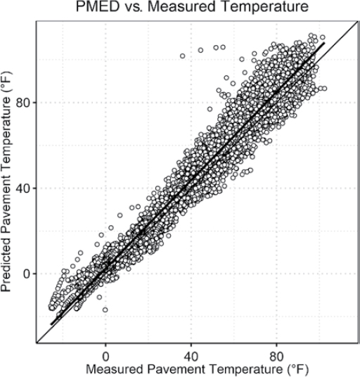

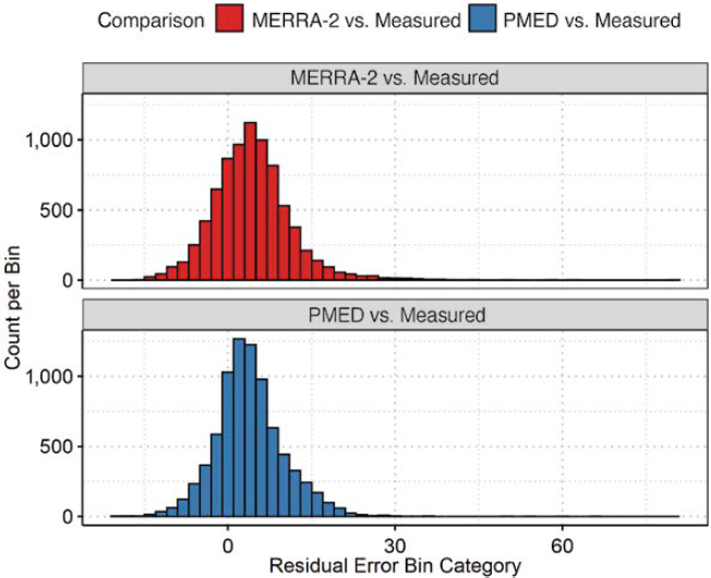
as the largest number of residual error observations fell within the first few positive bins (i.e., error values between 0 °F and 6 °F). The number of observations within these bins is greater for the current EICM/PMED method.
Linear Regression and Hypothesis Tests
The pairwise comparison, intercept, and slope hypothesis test results for the MERRA-2 and EICM/PMED comparisons with the measured pavement temperature data are summarized Tables 27 and 28, respectively. The mean difference between the measured and predicted pavement temperature was more than 3 °F for both cases, which quantifies the overprediction observed in Figures 25 and 26. The MERRA-2 case had a greater mean difference compared to the EICM/PMED dataset. The slope estimate was slightly greater than 1, with an intercept near 0 for the MERRA-2 case. For the EICM/PMED case, a slope equal to 1.03 and intercept of 2.49 was observed. All of the null hypotheses were rejected. Similar to the Arizona SMP site discussed previously, the results are not practically different from one another. For the Manitoba SMP site, the pavement temperatures predicted using the current EICM/PMED empirical method resulted in a slightly better prediction overall.
Table 27. MERRA-2 versus measured pavement temperature hypothesis test results for the Manitoba SMP site.
| Hypothesis Test | Value Estimate | P-Value |
|---|---|---|
| Paired t-test (mean difference) | –4.2968 | 0.0000 |
| Intercept = 0 | –0.6761 | 0.0000 |
| Slope = 1 | 1.1088 | 0.0000 |
Table 28. PMED-predicted pavement temperature versus measured pavement temperature hypothesis test results for the Manitoba SMP site.
| Hypothesis Test | Value Estimate | P-Value |
|---|---|---|
| Paired t-test (mean difference) | –3.8919 | 0.0000 |
| Intercept = 0 | 2.4906 | 0.0000 |
| Slope = 1 | 1.0307 | 0.0000 |
The hypothesis test results between the MERRA-2- and PMED-predicted pavement temperatures are summarized in Table 29. The average pairwise difference between the MERRA-2- and PMED-predicted pavement temperatures was less than 0.5 °F, which is practically insignificant even though the null hypothesis was rejected. The slope and intercept hypothesis tests were also found to be statistically significantly different, while the value estimates were practically the same as the null hypothesis.
RMSE, R2, and MRE
The overall error was analyzed by calculating the RMSE, R2, and MRE for each month within the dataset. Table 30 summarizes the monthly RMSE results for the Manitoba SMP site. Overall, the MERRA-2 dataset resulted in lower RMSE for 7 of the 12 months, especially for the non-summer months. The EICM/PMED method showed lower RMSE values for May through August. It was also observed that the RMSE values for the summer months were much greater than the non-summer months for both methods.
Table 31 shows the R2 calculated for each month, which showed a similar trend as the RMSE results. Table 32 summarizes the MRE for each month. The MRE provides additional information regarding the over or underprediction of pavement temperature compared to the measured values. The results show that the MERRA-2 showed consistent overpredictions of the measured pavement temperature in the summer months compared to the PMED-predicted pavement temperatures.
3.3.2.3 Georgia SMP Rigid
One-to-One Comparison
The measured and predicted pavement temperature results for the Georgia SMP site are shown in Figures 29 and 30. Overall, both figures show a linear trend along the line of equality.
Table 29. MERRA-2-predicted pavement temperature versus PMED-predicted pavement temperature hypothesis test results for the Manitoba SMP site.
| Hypothesis Test | Value Estimate | P-Value |
|---|---|---|
| Paired t-test (mean difference) | –0.4049 | 0.0000 |
| Intercept = 0 | –2.6547 | 0.0000 |
| Slope = 1 | 1.0617 | 0.0000 |
Table 30. Monthly RMSE for the Manitoba SMP site.
| Month | MERRA-2 vs. Measured | PMED vs. Measured |
|---|---|---|
| Jan | 5.6671 | 5.8833 |
| Feb | 5.1477 | 5.2050 |
| Mar | 5.9336 | 4.8380 |
| Apr | 7.1151 | 7.4873 |
| May | 10.0232 | 8.0472 |
| Jun | 11.4496 | 8.8364 |
| Jul | 13.6512 | 10.6845 |
| Aug | 10.7856 | 9.6286 |
| Sep | 8.1492 | 8.8387 |
| Oct | 5.9329 | 6.1718 |
| Nov | 3.7311 | 4.4478 |
| Dec | 3.5202 | 3.8112 |
Table 31. Monthly R2 for the Manitoba SMP site.
| Month | MERRA-2 vs. Measured | PMED vs. Measured |
|---|---|---|
| Jan | 0.74915 | 0.79200 |
| Feb | 0.86266 | 0.88451 |
| Mar | 0.73355 | 0.82737 |
| Apr | 0.81143 | 0.74304 |
| May | 0.71124 | 0.77340 |
| Jun | 0.67390 | 0.57939 |
| Jul | 0.54216 | 0.50311 |
| Aug | 0.69940 | 0.57866 |
| Sep | 0.84992 | 0.78370 |
| Oct | 0.80561 | 0.77469 |
| Nov | 0.84627 | 0.85824 |
| Dec | 0.87924 | 0.84097 |
Table 32. Monthly MRE for the Manitoba SMP site.
| Month | MERRA-2 vs. Measured | PMED vs. Measured |
|---|---|---|
| Jan | –1.61980 | –3.23759 |
| Feb | 1.68547 | –2.15505 |
| Mar | –0.93808 | –0.78334 |
| Apr | –4.05513 | –2.91052 |
| May | –6.48289 | –4.79631 |
| Jun | –9.04629 | –5.02854 |
| Jul | –10.94665 | –7.31495 |
| Aug | –8.42947 | –5.82500 |
| Sep | –6.73355 | –6.99886 |
| Oct | –4.53724 | –4.75415 |
| Nov | –1.08053 | –2.49417 |
| Dec | 1.09107 | –0.50313 |

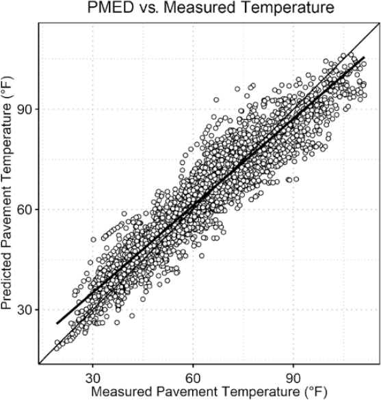
The MERRA-2-predicted pavement temperatures show a consistent positive bias for which the predicted temperatures were higher than the corresponding measured values. The scatter around the line of equality is greater for the MERRA-2 case compared to the EICM/PMED comparison. It should be noted that the Georgia SMP site did not have measured data for an entire year.
The MERRA-2-predicted pavement temperatures are plotted against the PMED-predicted pavement temperatures for the Georgia SMP site, as shown in Figure 31. The comparison shows a linear trend along the line of equality with lower scatter at lower temperatures compared to higher temperatures. It was also observed that at the higher temperature ranges above 100 °F, the MERRA-2-predicted temperatures were higher than those predicted using the PMED empirical equation.
Residual Error Histogram
The residual error was calculated for each hour the measured data were available. The number of observations within each residual error bin or group was counted to generate the histogram shown in Figure 32. The results show a positive bias for both cases, while the MERRA-2 comparison showed a greater bias compared to the EICM/PMED case. The EICM- and PMED-predicted pavement temperatures resulted in a better overall prediction of the measured pavement temperatures.
Linear Regression and Hypothesis Tests
The pairwise comparison, intercept, and slope hypothesis test results for the MERRA-2 and EICM/PMED comparisons with the measured pavement temperature data are summarized in Tables 33 and 34, respectively. The MERRA-2 case showed a greater mean difference between the predicted and measured pavement temperature compared to the EICM/PMED dataset. The slope estimate for the MERRA-2 case was closer to 1 and greater than the slope coefficient for the EICM/PMED comparison. The intercept was also lower for the MERRA-2 case. While the
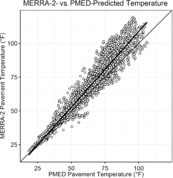
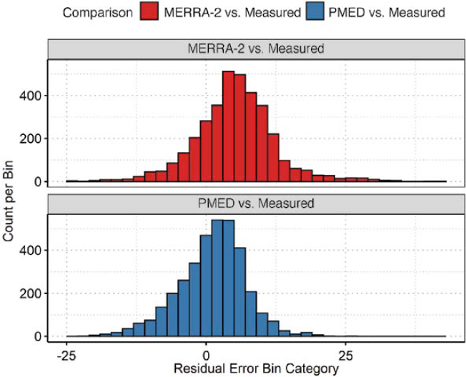
Table 33. MERRA-2 versus measured pavement temperature hypothesis test results for the Georgia SMP site.
| Hypothesis Test | Value Estimate | P-Value |
|---|---|---|
| Paired t-test (mean difference) | –5.2215 | 0.0000 |
| Intercept = 0 | 5.5025 | 0.0000 |
| Slope = 1 | 0.9954 | 0.4882 |
Table 34. PMED-predicted pavement temperature versus measured pavement temperature hypothesis test results for the Georgia SMP site.
| Hypothesis Test | Value Estimate | P-Value |
|---|---|---|
| Paired t-test (mean difference) | –1.0706 | 0.0000 |
| Intercept = 0 | 9.0868 | 0.0000 |
| Slope = 1 | 0.8678 | 0.0000 |
MERRA-2 case did result in better slope and intercept coefficients compared to the EICM/PMED comparison, the mean difference of more than −5 °F between the predicted and measured pavement temperatures makes the comparison slightly worse than the EICM/PMED case.
The hypothesis test results for the MERRA-2- versus PMED-predicted pavement temperatures comparison are summarized in Table 35. The average pairwise difference between the MERRA-2- and PMED-predicted pavement temperatures was greater than the Arizona and Manitoba SMP sites. On average, the PMED pavement temperatures were 4 °F lower than the MERRA-2predicted temperatures. The slope and intercept hypothesis tests were also statistically significantly different, while the value estimates were practically the same as the null hypothesis.
RMSE, R2, and MRE
The RMSE, R2, and MRE was calculated for the 5 months the measured data were available for the Georgia SMP site. Table 36 summarizes the RMSE results. Overall, the MERRA-2 dataset resulted in greater RMSE for all of the months compared to the EICM/PMED comparison. Table 37 shows the R2 calculated for each month and shows a similar trend as the RMSE results. Overall, the MERRA-2 data showed a worse prediction compared to the empirical calculations
Table 35. MERRA-2-predicted pavement temperature versus PMED-predicted pavement temperature hypothesis test results for the Georgia SMP site.
| Hypothesis Test | Value Estimate | P-Value |
|---|---|---|
| Paired t-test (mean difference) | –4.1509 | 0.0000 |
| Intercept = 0 | –3.4455 | 0.0000 |
| Slope = 1 | 1.1231 | 0.0000 |
Table 36. Monthly RMSE for the Georgia SMP site.
| Month | MERRA-2 vs. Measured | PMED vs. Measured |
|---|---|---|
| Jan | 7.7312 | 6.2100 |
| Feb | 5.8439 | 4.5027 |
| Mar | 9.1840 | 5.6659 |
| Apr | 9.8014 | 6.2361 |
| May | 11.3852 | 7.4934 |
Table 37. Monthly R2 for the Georgia SMP site.
| Month | MERRA-2 vs. Measured | PMED vs. Measured |
|---|---|---|
| Jan | 0.71898 | 0.78741 |
| Feb | 0.82924 | 0.88945 |
| Mar | 0.72979 | 0.85710 |
| Apr | 0.78388 | 0.83557 |
| May | 0.76111 | 0.77021 |
within the EICM and PMED. Table 38 summarizes the MRE for each month and shows the same trend as the RMSE and R2 results for which the MERRA-2 predictions were worse than the EICM/PMED predictions.
3.3.2.4 New Jersey SMP Flexible
One-to-One Comparison
The measured and predicted pavement temperature comparisons for the New Jersey SMP site are shown in Figures 33 and 34. The following observations were made:
- Both cases show a linear trend along the line of equality, with the MERRA-2 case showing more scatter around the line of equality compared to the EICM/PMED case.
- The scatter around the line of equality is less at lower pavement temperatures compared to the scatter at higher pavement temperatures.
- Overall, both cases compare fairly well against the measured pavement temperature values.
Table 38. Monthly MRE for the Georgia SMP site.
| Month | MERRA-2 vs. Measured | PMED vs. Measured |
|---|---|---|
| Jan | –3.5015 | –2.30595 |
| Feb | –2.5975 | –0.15162 |
| Mar | –4.4302 | –1.02785 |
| Apr | –6.9694 | 0.42888 |
| May | –8.7440 | –2.27230 |

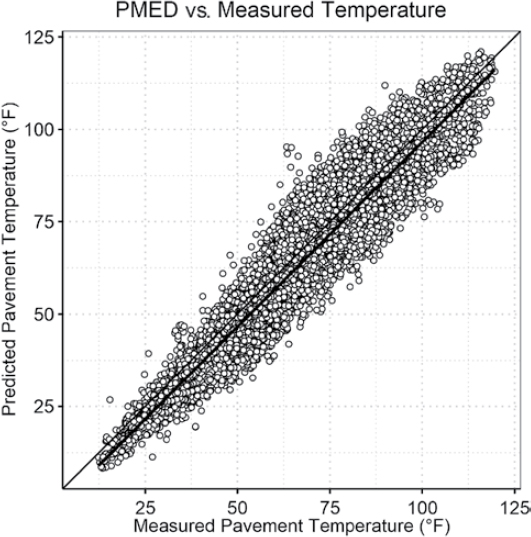
The MERRA-2-predicted pavement temperatures are plotted against the PMED-predicted pavement temperatures for the New Jersey SMP site, as shown in Figure 35. The comparison shows a linear trend along the line of equality with less scatter at lower temperatures compared to higher temperatures. Overall, the predicted pavement temperatures compare well with one another.
Residual Error Histogram
The residual error between the measured pavement temperature and MERRA-2- and EICM-predicted pavement temperatures was compared to help determine whether one method was better than the other. The residual error histogram is shown in Figure 36. The results show that the error distributions between the two cases are quite similar in that both show a negative bias. A larger number of observations within the first few bins to the left of 0 were observed for the MERRA-2 case.
Linear Regression and Hypothesis tests
The pairwise comparison, intercept, and slope hypothesis test results for the MERRA-2 and EICM/PMED comparisons with the measured pavement temperature data are summarized Tables 39 and 40, respectively. The following observations were made:
- The MERRA-2 case showed a lower mean difference (0.54 °F) compared to the EICM/PMED case (3.4 °F). Both cases were found significantly different than the null hypothesis.
- The MERRA-2 case resulted in a slope and intercept worse than the EICM/PMED case. However, the mean difference is more important in this case since it resulted in an indication of the average bias or over/underprediction of the measured values. The MERRA-2 case resulted in a slightly better prediction overall based on these results.
The hypothesis test results for the MERRA-2- versus PMED-predicted pavement temperatures comparison are summarized in Table 41. The average pairwise difference between the MERRA-2- and PMED-predicted pavement temperatures was greater than the Arizona and Manitoba

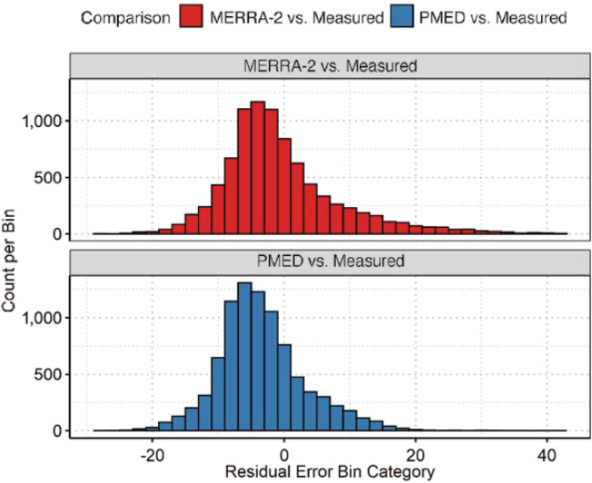
Table 39. MERRA-2 versus measured pavement temperature hypothesis test results for the New Jersey SMP site.
| Hypothesis Test | Value Estimate | P-Value |
|---|---|---|
| Paired t-test (mean difference) | 0.5450 | 0.0000 |
| Intercept = 0 | –4.8158 | 0.0000 |
| Slope = 1 | 1.0683 | 0.0000 |
Table 40. PMED-predicted pavement temperature versus measured pavement temperature hypothesis test results for the New Jersey SMP site.
| Hypothesis Test | Value Estimate | P-Value |
|---|---|---|
| Paired t-test (mean difference) | 3.4254 | 0.0000 |
| Intercept = 0 | –3.3968 | 0.0000 |
| Slope = 1 | 0.9995 | 0.8864 |
Table 41. MERRA-2-predicted pavement temperature versus PMED-predicted pavement temperature hypothesis test results for the New Jersey SMP site.
| Hypothesis Test | Value Estimate | P-Value |
|---|---|---|
| Paired t-test (mean difference) | –2.8804 | 0.0000 |
| Intercept = 0 | –0.4584 | 0.0177 |
| Slope = 1 | 1.0565 | 0.0000 |
SMP sites and less than the Georgia SMP site. On average, the PMED pavement temperatures were almost 3 °F lower than the MERRA-2-predicted temperature. The slope and intercept hypothesis tests were also statistically significantly different, while the value estimates were practically the same as the null hypothesis. Overall, the MERRA-2- and PMED-predicted pavement temperatures are in good agreement.
RMSE, R2, and MRE
The RMSE, R2, and MRE were calculated for each month the data were available. Table 42 summarizes the RMSE results for the New Jersey SMP site. Overall, the results show very similar RMSE values for January through March and October through December. The EICM/PMED case showed lower RMSE values between April and September, which corresponds well with the one-to-one comparisons shown in Figure 34.
Table 43 shows the R2 calculated for each month, which showed that the EICM/PMED case had greater R2 for most of the months. Some of the R2 values were much lower compared to the other SMP sites included in the analysis.
Table 44 summarizes the MRE for each month. The results show that the MERRA-2 resulted in higher MRE values compared to the PMED-predicted temperatures.
Table 42. Monthly RMSE for the New Jersey SMP site.
| Month | MERRA-2 vs. Measured | PMED vs. Measured |
|---|---|---|
| Jan | 5.8190 | 4.9189 |
| Feb | 6.5013 | 6.6007 |
| Mar | 8.1384 | 8.3976 |
| Apr | 9.2945 | 6.6624 |
| May | 13.1989 | 8.3404 |
| Jun | 11.0977 | 8.3437 |
| Jul | 10.3199 | 8.0400 |
| Aug | 9.3111 | 8.2301 |
| Sep | 8.2187 | 6.5433 |
| Oct | 7.2920 | 7.2667 |
| Nov | 7.6641 | 6.9412 |
| Dec | 8.0484 | 7.7004 |
Table 43. Monthly R2 for the New Jersey SMP site.
| Month | MERRA-2 vs. Measured | PMED vs. Measured |
|---|---|---|
| Jan | 0.78041 | 0.85902 |
| Feb | 0.62763 | 0.73319 |
| Mar | 0.76379 | 0.84519 |
| Apr | 0.69023 | 0.89584 |
| May | 0.44842 | 0.55755 |
| Jun | 0.66984 | 0.71744 |
| Jul | 0.63106 | 0.68083 |
| Aug | 0.59732 | 0.61735 |
| Sep | 0.57300 | 0.75560 |
| Oct | 0.73847 | 0.72264 |
| Nov | 0.75760 | 0.81876 |
| Dec | 0.75236 | 0.80613 |
3.3.3 Summary
In summary, the validation results using a subset of LTPP SMP sites showed generally good agreement between the measured and predicted pavement temperature regardless of which method was used. The following items were highlighted:
- Using the MERRA-2 shortwave and longwave radiation directly to calculate pavement temperature did not always result in a better prediction compared to the measured data.
Table 44. Monthly MRE for the New Jersey SMP site.
| Month | MERRA-2 vs. Measured | PMED vs. Measured |
|---|---|---|
| Jan | 3.9614500 | 3.53832 |
| Feb | 2.0303626 | 4.58406 |
| Mar | 2.6076283 | 5.90310 |
| Apr | –0.0093315 | 4.12581 |
| May | –6.2889462 | 0.98563 |
| Jun | –5.3467703 | 0.23912 |
| Jul | –3.9345237 | 1.64100 |
| Aug | –1.9039480 | 3.58046 |
| Sep | 0.3489081 | 1.80377 |
| Oct | 3.7589060 | 3.36164 |
| Nov | 5.3686729 | 5.09044 |
| Dec | 6.5289736 | 6.48269 |
- At higher pavement temperatures, larger differences between the measured and predicted pavement temperatures were observed. It is possible that using only the shortwave and longwave radiation variables in the energy balance equation does not capture the true behavior at the pavement surface and is missing another variable, such as sensible heat, ground heat, or latent heat effects.
- Potential items that could help explain some of the larger differences include the following:
- – Localized weather events, unique terrain, and ground cover types around the specific SMP site may not be captured well within the assimilated MERRA-2 dataset. Even though the MERRA-2 data were modeled and validated using atmospheric and ground-based data, it cannot account for everything.
- – Sensible heat, latent heat, and ground heat effects were not included in the overall energy balance calculations and could have a significant effect. The amount of sensible heat, latent heat, and ground heat is dependent on the location. One variable could have a much larger impact in the dry non-freeze locations compared to a wet-freeze region.
- The MERRA-2 shortwave and longwave radiation data should be included in the hourly climate data imported into the EICM/PMED. The empirically calculated shortwave and longwave radiation regression equation was derived using data predominantly from the Midwestern United States and assumed to apply to all locations, which is not an accurate assumption.
3.4 Identifying Enhancements to Improve EICM Functionality and Maintainability
The EICM was originally developed using the FORTRAN software language. The source code was compiled into a standalone executable, which was then used by other software applications, such as the MEPDG MOP developed as part of NCHRP Project 1-37A, “Development of the 2002 Guide for the Design of New and Rehabilitated Pavement Structures: Phase II” and all versions of the PMED software developed by AASHTOWare until the release of version 2.5 (v2.5) in 2018. With the release of PMED v2.5, all FORTRAN and C++ source code was transliterated to the C# language. Using a single language throughout the application was vital to ensure the software remains maintainable and adhere to modern software development standards and practices. Many of the FORTRAN and C++ libraries used in the original source code have not been maintained or are not available anymore. The transliteration process was completed line by line to ensure the results are near identical to the non-C# versions. This process did not attempt to improve the functionality or run-time of the EICM. Several enhancements were identified to improve the EICM documentation, maintainability, and analysis run-time of the EICM.
3.4.1 EICM Documentation
Detailed information regarding the documentation of the EICM source code modules and subroutines are not well defined in literature. The current EICM has undergone several changes and revisions since its original development by Dempsey et al. (3), which were developed throughout several research studies. A major enhancement to the overall use of environmental data within pavement analysis and design and the EICM is to prepare a detailed reference manual that describes the EICM model input variables and properties, assumptions, limitations, model equations, and predicted outputs. The major topics for the reference manual are listed here:
- Pavement configuration and boundary conditions
- – General inputs, constants, and boundary conditions
- – Pavement layer information, such as number of layers, material types, thicknesses, and sublayering methods
- – Site-specific information, such as hourly climate data, and water table depths
- – Structural, thermal, and moisture material properties
- Climatic models
- – Temperature model
- – Moisture model
- – Material model
- Outputs
- – Thermal and moisture outputs
- – Material stiffness output
3.4.1.1 Pavement Configuration and Boundary Conditions
The EICM requires many inputs, which are required for certain features to work as intended. Many of these inputs are not adjustable in the EICM’s current form. Table 45 summarizes the constant inputs or settings within the EICM.
Available Layer Types
The following pavement material layer types can be modeled in the current EICM:
- Asphalt concrete
- Portland cement concrete
Table 45. Common inputs and assumptions for all analysis types within the EICM.
| Input Variable | Assumed or Default Values | Units |
|---|---|---|
| Total depth | 360 | in |
| Initial nodal temperature | Assumed as the MAAT | ºF or ºC |
| Constant temperature of last layer | Set as the MAAT | ºF or ºC |
| Upper temperature limit of freezing range in which water is partially frozen and unfrozen | 32 | ºF |
| Lower temperature limit of freezing range | 30.2 | ºF |
| Maximum allowable convection coefficient | Hard coded to 3 | BTU / h – ft2 –ºF |
| Analysis time step | 0.1 | h |
| Time step for analysis outputs | 1 | h |
| Emissivity factor | 0.93 | |
| Longwave back radiation factor | 0.77 | |
| Geiger longwave radiation factor | 0.28 | |
| Rho factor | 0.074 | |
| Vapor pressure of atmosphere near surface | Hard coded to 5 | mmHg |
| Time of day when minimum temperature occurs | 4.0 (4 am) | |
| Time of day when maximum temperature occurs | 15.0 (3 pm) | |
| Water table depth | User defined | ft or m |
- Stabilized or treated base
- Unbound aggregate base
- Subgrade soils
- Bedrock
Sublayering and Nodal Spacing Within the EICM. The EICM divides the pavement-base-subgrade structure into sublayers up to a depth of 360 in. The specific details for each layer type are listed here:
- Asphalt and stabilized base materials
- – If the layer thickness is less than or equal to 1.5 in, a single sublayer is used.
- – If the layer thickness is greater than 1.5 in and less than or equal to 2 in, two sublayers are used.
- – If the layer thickness is greater than 2 in, the layer is divided into 1-in sublayers. For example, for a 6-in asphalt layer, six 1-in sublayers will be present.
- Portland cement concrete (PCC) materials
- – If the PCC layer is less than or equal to 2 in, a total of two sublayers is used.
- – For all other thicknesses, the total PCC layer thickness is divided by 0.875 in to determine the total number of sublayers for the PCC layer.
- – For example, a 9-in PCC layer will be subdivided into a total of 10 sublayers. The calculation is as follows: 9/0.875 = 10.28 = 10.
- Non-stabilized unbound base materials
- – If the total layer thickness is less than or equal to 2 in, then a single sublayer is used.
- – Otherwise, the total layer thickness is divided into 2-in sublayers, except for PCC designs. If the layer is not divisible by 2, any remainder thicknesses will be added to the last sublayer to ensure the minimum sublayer thickness for a non-stabilized unbound base material is not less than 2 in.
- – For example, a 12-in unbound base material will be divided into six 2-in sublayers.
- – For PCC designs, the unbound base layers are divided into 4-in sublayers.
- Subgrade soils
- – First, the total thickness of the layers above the subgrade is calculated. Second, the total subgrade depth is calculated by subtracting the total thickness of the layers above the subgrade from 360 in.
- – For example, assuming the asphalt layer and unbound base layer thicknesses are 6 and 12 in, respectively, the total subgrade thickness is 360 in − 18 in, which is equal to 342 in.
- – The total number of sublayers for the subgrade is calculated based on the depth from the bottom of the last unbound base layer to a depth of 360 in, which is divided by 6 in, except for PCC designs, to determine the total number of sublayers. For the example presented above, the subgrade will be divided into 57 6-in sublayers or nodal elements.
- – For PCC designs, the subgrade thickness from the bottom of the base layer to the semi-infinite boundary condition of 360 in is divided into 4-in sublayers.
- The results from the sublayering process are included in the EICM input file.
- It should be noted that the number of sublayers for each material is based on integer values.
- Within the main subroutine, additional sublayer modifications are performed to conform with the requirements of the rigid and flexible pavement distress and performance prediction models.
Common Inputs for All Analysis Types
The hourly climate inputs required by the EICM are summarized in Table 46. Additional variables calculated from the hourly input data include daily, monthly, and yearly averages; wet days; freezing index; and freeze-thaw cycles.
Table 46. Common hourly climate inputs for all analysis types within the EICM.
| Hourly Climate Input | Units |
|---|---|
| Air Temperature | °F or °C |
| Wind Speed | m/h or km/h |
| Percent Sunshine | % |
| Precipitation | in or mm |
| Relative Humidity | % |
Material-Specific Inputs
- Asphalt and Portland cement concrete layers
- – Layer thickness
- – Unit weight
- – Thermal conductivity
- Unbound aggregate base materials and subgrade soils
- – Resilient modulus: Direct input (psi or MPa)
- Frozen modulus: not a direct input
- Unfrozen modulus: assumed equal to resilient modulus input
- – Optimum volumetric water content: direct input or calculated (%)
- – Soil water characteristic curve
- Fredlund (a) factor: Calculated
- Fredlund (b) factor: Calculated
- Fredlund (c) factor: Calculated
- Fredlund (hr) factor: Calculated
- – PI: Direct input (%)
- – Grain size distribution-related inputs
- Passing #200 sieve: Direct input (%)
- Passing #4 sieve: Direct input (%)
- D60(mm), grain size diameter corresponding to 60% passing: Calculated
- – Porosity: Calculated (%)
- – Saturated permeability or hydraulic conductivity: Direct input or calculated (ft/h or m/h)
- – Initial volumetric water content: Calculated (%)
- – Thermal conductivity: 0.23 (BTU/h − ft − °F or W/m2)
- Adjusted internally based on temperature and moisture content
- – Heat capacity: 0.17 (BTU/lb − °F or J/kg − K)
- Adjusted internally based on temperature and moisture content
- – Resilient modulus: Direct input (psi or MPa)
- Bedrock
- – Constant modulus (psi or MPa)
Calculated Material Properties Based on Inputs
Mass-Volume Parameters
Optimum Gravimetric Water Content, wopt (%). For non-plastic granular materials, the following equations are used to calculate the optimum gravimetric water content.
When wPI = 0, where wPI is a weighted plasticity index determined by multiplying the PI by the percent passing of the #200 sieve (P200). The gravimetric water content is estimated using the following relationship:
For plastic unbound materials, the following equations are used to calculate the optimum gravimetric water content:
If PI > PIadj, then use PIadj
If PI ≤ PIadj, then PIadj = PI
Optimum Volumetric Water Content, θopt
where the unit weight of water is represented by γw = 62.4 lb/ft3
Maximum Dry Unit Weight, γdmax.
For non-plastic granular materials when wPI = 0,
where Gs is the specific gravity of solids and Sopt is the initial degree of saturation based on optimum moisture conditions. For plastic soils, different equations are used based on whether the material is compacted. If the layer is compacted, the following equation is used to determine the maximum dry density:
If the material is not compacted, the following equation is used:
Specific Gravity of Solids, Gs. The specific gravity of solids uses a value of 2.7 by default and can also be specified directly by the user.
D60. The grain size diameter corresponding to 60% passing is calculated based on the percent passing of individual sieve sizes.
Initial Degree of Saturation, Sopt. If the maximum dry density input is defined by the user and not internally calculated, and not using the regression equations, then the Sopt is calculated using the following equation:
For non-plastic granular materials, when wPI = 0, the initial degree of saturation at optimum moisture conditions are determined using the following equation:
Sopt = −100.17 + 1.4991 × P2-in + 0.56155 × P1-in − 0.36755 × P0.5
In all other cases, the value is set to Sopt = 60.
Porosity. The porosity is defined as the ratio between the volume of voids to the total volume from the weight/mass and volume relationship. Based on the known quantities at the time of the analysis, the porosity is calculated using the following equation:
Saturated Hydraulic Conductivity, ksat. For non-plastic granular materials and when wPI = 0, the following equation is used to estimate the saturated hydraulic conductivity:
ksat= 10−6 × 105.3×D10+0.049×D10+0.0092×(D60/D10)−0.1×P200+1.5
Additionally, if ksat > 10, then it is set to a value of 10. For plastic soils, the following equation is used to estimate the saturated hydraulic conductivity with units of cm/s:
ksat = 107.014−0.0376×LL−0.361×γd−7.932×Log(PI)+0.249×γd×PI0.105
The saturated hydraulic conductivity undergoes a unit conversion internally from cm/s to ft/h, 1 cm/s = 118.11023 ft/h.
SWCC Parameters. The Fredlund and Xing method was implemented in the EICM to determine the SWCC-related parameters. The regression equations derived for each parameter are dependent on the soil type.
For plastic soils, the following equations are used to determine the various Fredlund and Xing factors:
Fredlund (a) Factor
af = 32.835 × Ln(wPI) + 32.438
- If af < 5, then af = 5
Fredlund (b) Factor
bf = 1.421 × wPI−0.3185
Fredlund (c) Factor
cf = −0.2154 × Ln(wPI) + 0.7145
- If cf < 0.01, then cf = 0.03
Fredlund (hr) Factor
hrf = 500
wPI = P200 × PI
For non-plastic soils, the following equations are used to determine the Fredlund and Xing factors:
Fredlund (a) Factor
- If af < 1, then
- NCHRP Project 09-23 reports an additional calculation not present in the EICM source code (10). The af factor above includes one additional step: af = 1.14 × a − 0.5. It is unclear why this step was omitted from the EICM.
Fredlund (b) Factor
bf = 0.936 × b − 3.8
- If bf < 0.3, then bf = 0.3, and if bf > 4, then bf = 4.
Fredlund (c) Factor
cf = 0.26 × e0.748 × c + 1.4 × D10
- NCHRP Report 602: Calibration and Validation of the Enhanced Integrated Climatic Model for Pavement Design (10, 16) documents that the exponent in the cf is 0.758 and not 0.748. It is unclear whether the change is intentional or a typo.
Fredlund (hr) Factor
hrf = 100
Saturated Permeability or Hydraulic Conductivity
- Direct input or calculated value in ft/h or m/h
3.4.1.2 EICM Climate Models
Energy Balance Near the Ground Surface
The following energy balance equations are used to calculate the climatic and radiation data for each time increment for the given day and hour. The subroutine within the EICM calculates the net shortwave radiation, net longwave radiation, net total radiation, and convection coefficient.
Shortwave Radiation
- Net Shortwave Radiation
Qs = Qi − Qr
where Qi is the incoming shortwave radiation and Qr is the reflected shortwave radiation.
where αs is the surface shortwave absorptivity of the pavement surface, Rn is the extraterrestrial radiation incident on a surface normal to the direction of the sun, A and B are constants that account for diffuse scattering and adsorption by the atmosphere, and Sc is the percentage of sunshine.
Longwave Radiation. Net longwave radiation is a function of incoming or absorbed longwave radiation from the atmosphere and outgoing or emitted longwave radiation by the Earth’s surface. The net longwave radiation is calculated using the following equation:
Ql = Qa − Qe
where Qa is the incoming or absorbed longwave radiation and Qe is the longwave radiation emitted by the surface.
where σ is the Stefan-Boltzman constant; є is the atmospheric emissivity; Tair is the air temperature in degrees Rankine; ρ is the vapor pressure of air hard coded to a value of 5 mmHg; G, J, and P are
dimensionless constants; Ts is the pavement surface temperature in degrees Rankine; N is the cloud base factor; and W is the average cloud cover equal to 1 − Sc.
Heat Transfer by Convection. The heat transfer due to convection at the Earth’s surface is calculated using the following equation:
Qc = H(Tair − T1)
The convection coefficient, H, computed using an empirical equation developed by Vehrencamp (14) and reported by Dempsey et al. (3), is shown here:
where Vm is the average of the air temperature and pavement surface temperature in K, Uwind is the wind velocity in mph converted to m/s (1 mph = 0.447 m/s), T1 is the surface temperature in °C, and Tair is the air temperature in °C. The value of 122.93 converts the units from g − cal/min − cm2 − °C to BTU/h − ft2 − °F. The wind velocity input in the EICM is in mph and converted to m/s, hence the 0.447 multiplier in the equation. The value of 1.33 is not well defined and is of an unknown origin. The maximum allowed convection coefficient is a hard-coded value set to 3.0 BTU/h − ft2 − °F. The value was selected to ensure stability within the analysis module when the analysis increments are large. The EICM within the PMED uses an analysis increment of 0.1 h, which is short enough to not cause stability issues. Therefore, the maximum convection coefficient can be adjusted.
Pavement Temperature
The pavement temperature is adjusted for each node throughout the pavement structure, starting from the pavement surface. The calculations are performed for the different node types (i.e., surface, interface, and interior) and node states (i.e., unfrozen, freezing, or frozen). It should be noted that the state of the node is calculated for each time increment and the different node types. The boundary conditions to determine the state of the node are defined here:
- Boundary conditions:
- – Top temperature of freezing range: 32 °F
- – Bottom temperature of freezing range: 30 °F
- Unfrozen conditions:
- – When the temperature is greater than or equal to the top temperature of the freezing range Tnode ≥ 32 °F
- – If the adjusted temperature is less than the top temperature of the freezing range, the nodal temperature is set to the top temperature minus 0.01 to consider latent heat effects.
- – Another check is in place to determine whether the adjusted nodal temperature is below the bottom temperature of the freezing range or between the two limits.
- Frozen conditions:
- – Temperature is less than the top temperature of the freezing range, Tnode < 32 °F
- Freezing conditions:
- – 30 °F < Tnode < 32 °F
General Form of the One-Dimensional, Fourier Equation for Conductive Heat Transfer
General equation:
With finite difference terms:
where Tn is the temperature of the current node, Tn–1 is the temperature of the previous node, Tn+1 is the temperature of the next node, and α is the thermal diffusivity and equal to .
The terms within the general equation are applied to account for the different nodal interfaces within the pavement structure. The calculations are applied at the pavement surface location, interior nodal locations where the material properties are the same, and at interface locations where different layer types are accounted for.
At the Pavement Surface. The finite difference equation for nodal locations at the pavement surface is shown here:
where k represents the hydraulic conductivity, T1 and T2 are the temperature of node 1 and node 2, Tair is the air temperature, Qrad is the total net radiation (shortwave and longwave), γ is the unit weight, c is the thermal conductivity of the layer, ΔX is the distance between nodes, Δθ is the time step increment, and is the calculated future temperature for the current node. The equation is rearranged to solve for the future surface temperature of time increment Δθ:
At Interior Locations. Similar to the surface locations, the following equation is used to determine the temperature for interior locations:
The equation is rearranged to solve for the future nodal temperature:
At Interface Nodes Between Two Materials. For nodal locations at the interface between two materials, the material properties of both layers are required to determine the nodal temperature. The following equations are used for nodal locations at the interface between two materials:
where
Additional Explanation of Terms. The thermal conductivity of a nodal volume is represented by:
The heat storage in a nodal volume during an incremental time period, Δθ, is represented by:
Stability Checks
Stability checks are performed for each node type (i.e., surface, interior, and interface) and node state (i.e., thawed, freezing, and frozen). The main stability assumption is that all temperature coefficients must be positive. The stability checks are presented here:
Surface Node
Interior Node
Interface Node
Moisture and Temperature Models
The moisture model adjusts the unbound base and natural subgrade material moisture conditions on an hourly basis. The calculations are presented in the following section.
Hourly Changes Within the EICM. The default time step within the hourly analysis is 0.1 h. The following computations are performed for each hour and include unit conversions between the units of the input variable and what the calculation expects since they are not always the same throughout the EICM:
Hourly Calculation Step 1 – Convert Units for Temperature, Pore Pressure, and Nodal Depths
- Temperature values are converted from °F to °C.
- Pore pressure is converted from psi to cm head.
- Nodal depths are converted from in to cm.
Hourly Calculation Step 2 – Convert Units for Density, Nodal Elements, Saturated Hydraulic Conductivity, and Thermal Conductivity
- Density is converted from lb/ft3 to g/cm3.
- – 1 lb/ft3 = 0.01601873 g/cm3
- Nodal element incremental steps are converted from in to cm.
- – 1 in = 2.54 cm
- Saturated hydraulic conductivity is converted from ft/h to cm/h.
- – 1 ft/h = 30.48 cm/h
- Thermal conductivity is converted from BTU/h – ft – °F to cal/h – cm – °C.
- – 1 BTU/h – ft – °F = 14.9 cal/h – cm – °C
Hourly Calculation Step 3 – Calculate the Distance from Current Node to the Water Table Depth
- The water table depth is converted from ft to cm.
- This step calculates the suction head in cm if the water table depth is above the current nodal depth.
- The suction head is in units of cm of water head.
- – 1 cm of head = 10.197 kPa
Hourly Calculation Step 4 – Calculate the Base and Subgrade Layer Suction Values Based on Daily TMI. The base layer matric suction is calculated using methods described in NCHRP Project 09-23 using derived regression equations as a function of the TMI, P200, and PI. The weighted PI is calculated by multiplying the P200 value by the PI, as shown later. It should be noted that if the base layer P200 is greater than 2%, then it is set equal to 2%:
The base layer volumetric water content is determined by the following equation:
Additional adjustments are set in place when θbase > 40. For these cases, the volumetric water content is determined by the following equation:
θbase = 40 + 0.11 × P200 − 53
When θbase > θsat, then θbase = θsat.
Finally, the matric suction within the base layer is calculated based on the volumetric water content and converted from kPa to cm of water head.
- 1 cm head = 0.09804 kPa
The subgrade suction is calculated at a location 48 in below the last bound layer when the water table sits below 48 in.
Hourly Calculation Step 5 – Adjust the Latent Heat Budget of Water. This step calculates the latent heat budget of water when freezing. The maximum available latent heat is 80 cal/g or 80 cal/cm3 multiplied by the water content:
LHwater = 80 × wopt
Hourly Calculation Step 6 – Adjust the Hydraulic Conductivity Values Based on Moisture and Temperature States. This step calculates:
- Average pore pressure or cm head between node “n” and node “n+1”
- – If pore pressure or cm head is positive or below the depth of the water table, then no adjustments need to be made to the saturated hydraulic conductivity.
- – If the node is above the water table, then adjust the saturated hydraulic conductivity to an unsaturated hydraulic conductivity value.
- Average temperature between node “n” and node “n+1”
- – If the soil is in a freezing condition, but not yet frozen, then the freezing pore pressure is calculated using the following equation:
- Saturated hydraulic conductivity is multiplied by a permeability reduction factor.
Hourly Calculation Step 7 – Calculate the Slope of SWCC
- The slope of the SWCC for the current moisture and temperature conditions is calculated. The values are interpolated between the water content and suction differences.
Hourly Calculation Step 8 – Adjust the Thermal Conductivity Based on the Moisture and Temperature States. This step documents the adjustments to dry and saturated thermal conductivity for frozen and unfrozen conditions.
Kersten’s number:
For fine grained unfrozen soils,
Ke ![]() log(Sr) + 1
log(Sr) + 1
For coarse grained unfrozen soils,
Ke ![]() 0.7log(Sr) + 1
0.7log(Sr) + 1
where Sr is the degree of saturation
Dry thermal conductivity:
where γd is the dry density in kg/m3. For crushed materials where D60 > 10, the dry thermal conductivity is calculated as a function of porosity and shown in the following equation:
kdry = 0.39 × n−2.2
Saturated thermal conductivity for frozen and unfrozen conditions:
- Unfrozen conditions
where ks is assumed as 4 W/m-K and hard coded within the EICM, kw is assumed as 0.57 W/m-K and hard coded within the EICM, and n is the porosity.
- Frozen conditions
where ki is the thermal conductivity of ice and assumed as 2.2 W/m-K and wu is the fraction of unfrozen water. The equation can be reduced to the following equation:
Unsaturated thermal conductivity:
kunsat = (ksat − kdry) × Ke + kdry
In summary:
- Adjustments to thermal conductivity for dry, saturated, and unsaturated conditions and frozen or unfrozen soils are calculated in W/m-K and converted to cal/cm − h − °C for the subsequent calculations. The conversion from W/m-K to cal/cm − h − °C is as follows:
- – W/m-K is divided by 1.73073 to get BTU/h − ft − °F and then multiplied by 14.9 to get cal/cm − h − °C.
- The equations presented in this section were obtained from the source code and mostly based on the relationships developed by Johansen as reported by Farouki (17).
Hourly Calculation Step 9 – Calculate the Apparent Heat Capacity for Current Conditions. The heat capacity changes as a function of water content, quantity of ice, density, and heat capacity of water and soils. The following equations within the EICM calculate the apparent heat capacity for each hour:
where
- γice = 0.917 g/cm3 is unit weight of ice.
- γw = 1 g/cm3 is the unit weight of water.
- cice = 0.55 cal/cm3 − °C is the heat capacity of ice.
- cw = 1.0 cal/g − °C is the heat capacity of water.
- cs = cal/g − °C is the heat capacity of the soil.
Hourly Calculation Step 10 – Calculate the Convective Heat Flux. This step calculates the convective heat flux for the hourly nodal domain boundary per CRREL frost model.
Hourly Calculation Step 11 – Calculate the Check for Maximum Convective Heat Flux. This step determines whether the convective heat flux exceeds the maximum value.
Hourly Calculation Step 12 – Compute the Final Moisture and Temperature Adjustments. The remaining steps in the hourly calculation are related to the finite difference method described previously for each time increment and nodal depths:
- For each node, update the total nodal density to account for moisture and temperature state.
- Update available latent heat of water in soil layers based on moisture and temperature state.
- Update nodal temperature to account for moisture and temperature state.
- Determine the unfrozen/frozen/freezing condition of each node throughout the structure and determine freezing and thawing depths.
- Convert units back to original form required outside of the hourly loops.
- Continue to day loop.
Daily Calculations. The EICM calculates the following daily adjustments:
- Modulus adjustment factors for each layer and sublayer.
- Moisture content for each layer and sublayer.
- Quantile temperatures for asphalt layers.
- – The quantile temperatures calculations are not directly consumed by the EICM. The source code includes the calculations, while it is only used by the asphalt distress prediction models.
Modulus Adjustments
MR = FEnv × MRopt
Resilient Modulus of Unbound Layers for Frozen Conditions. If the temperature within an unbound layer is below freezing, the EICM calculates FEnv based on the Frozen Resilient Modulus (MRfrz), which is given as:
where P200 is the percent passing of the #200 sieve of the unbound material and PI is the plasticity index. Using the above MRfrz, the adjustment factor under freezing conditions is simply calculated as follows:
Resilient Modulus of Unbound Layers for Unfrozen Conditions Stability Checks. If the temperature within the unbound layer is above 32 °F, the adjustment factor FEnv is calculated as a function of moisture. More specifically, the equation for the adjustment factor is given as:
where S is the degree of saturation expressed in decimal; Sopt is the optimum degree of saturation also expressed in decimal; and a, b, and km are regression parameters for both coarse-grained and fine-grained materials. It should be noted that the a and b parameters define the minimum and maximum values of log(FEnv), respectively.
- Parameter fine-grained materials (P200 less than 50)
- – a = −0.3123
- – b = 0.3
- – km = 6.8157
- Coarse-grained materials
- – a = −0.5934
- – b = 0.4
- – km = 6.1324
Resilient Modulus of Unbound Layers for Recovering Conditions. For unbound materials under thawing (or recovering) conditions, the adjustment factor is first calculated for normal, unfrozen conditions and is multiplied by an additional correction factor. More specifically,
FEnv = FUnfrz × Crec
where FUnfrz is the adjustment factor for unfrozen materials calculated by substituting FUnfrz in place of FEnv and Crec is the correction factor for the recovering material calculated as follows:
Crec = RF + (1 − RF) × RR
where RF is the MR reduction factor and RR is the recovery ratio that can range from 0 (for “immediately after thawing” condition) to 1 (for “fully recovered” condition). The values of RF for coarse-grained and fine-grained materials are given in Tables 47 and 48, respectively.
The RR for unbound materials under thawing conditions is obtained using the following equation:
Table 47. Modulus reduction factor, RF, for different fractions of coarse-grained materials.
| Fraction of Coarse Material | P200 (%) | PI < 12% | 12% < PI ≤ 35% | PI > 35% |
|---|---|---|---|---|
| Mostly Gravel (P_4 < 50%) | < 6 | 0.85 | - | - |
| 6–12 | 0.65 | 0.70 | 0.75 | |
| >12 | 0.60 | 0.65 | 0.70 | |
| Mostly Sand (P_4 > 50%) | < 6 | 0.75 | - | - |
| 6–12 | 0.60 | 0.65 | 0.70 | |
| >12 | 0.50 | 0.55 | 0.60 |
Table 48. Modulus reduction factor, RF, for fine-grained materials (P200 > 50%).
| P200 (%) | PI < 12% | 12% < PI ≤ 35% | PI > 35% |
|---|---|---|---|
| 50–85 | 0.45 | 0.55 | 0.60 |
| >85 | 0.40 | 0.50 | 0.55 |
where Δt is time elapsed since thawing started in days and TR is the recovery period given as follows:
It should be noted that if RR = 0, then Crec = RF, which is always less than 1.0, and hence FEnv < FUnfrz (i.e., the resilient modulus of the recovering material is always less than the unfrozen material). On the other hand, if RR = 1, then Crec = 1, which makes FUnfrz = FEnv. In other words, the resilient modulus of the fully thawed material is equal to the modulus of unfrozen material.
3.4.2 Other Improvements
3.4.2.1 Input File and Run-Time Improvements
The EICM input text file (input.tmp) contains the required data to successfully execute the analysis. The structure of the current text file is very difficult to read and to identify what each variable or value means. Additionally, the file contains of a mix of comma and tab-separated values throughout and includes values not used in any of the EICM analysis modules.
The following improvements are recommended:
- Update the input file to a consistent format, such as JSON, XML, or delimited text.
- Provide input data dictionary for each input variable and their description.
- Remove input variables not used in the EICM.
-
Remove any inputs, code, flags that are always constant, such as:
- – Daily temperature output flag,
- – SWCC function type (Gardner or Fredlund), and
- – Time of minimum and maximum air temperature.
This input was only required when hourly data were not available. Estimating hourly data from minimum and maximum values is not needed with the availability of MERRA-2 data.
- If the new hourly shortwave and longwave radiation variables from MERRA-2 are used, include an option or flag to bypass the hard-coded inputs to the shortwave and longwave radiation empirical equations. To ensure backwards compatibility, incorporate the deprecated inputs as their own data class for the EICM. The following inputs and hard-coded values will be deprecated:
- – Longwave and shortwave radiation empirical methods,
- – Calculations for sunrise and sunset, and
- – Extraterrestrial solar radiation based on location and solar declination angle.
- Adjust the values that set the constant deep ground temperature lower boundary condition to accommodate areas where the MAAT is less than 32 °F/0 °C. It is recommended to include additional methods to set the initial nodal temperatures to a user-defined value, a mean monthly temperature at the start of the analysis period, or a constant value above freezing.
- Add new variables and values based on the findings and suggestions from this research project.
3.4.2.2 Run-Time Enhancements
The EICM is one of the most time-consuming analysis modules in the PMED. The analysis computations are performed every six minutes throughout the specified design life at various depths throughout the pavement layer structure. Improving the analysis run-time with the current EICM is very difficult without performing a complete refactor to bring the software up to modern software engineering standards. Additional considerations include using parallel analysis processes to perform some of the calculations simultaneously.
3.4.2.3 Output of Analysis Modules
The current version of the EICM produces several intermediate output files, which can be consumed by other models within the PMED software or other applications. Many of these files are poorly formatted or documented and only represent a small number of the data calculations included in the EICM. The research team suggested that an option be made available to customize what the EICM produces as outputs, which can then be consumed by other products or software. The following steps are recommended to improve the format and usability of the outputs from the EICM:
- Select a consistent file format for all generated output files.
- – The current EICM output files are a series of text files with different formatting, file extensions, and delimiters. A consistent format should be selected and documented. Example file formats include, JSON, TXT, CSV, TSV, and XML.
- Add additional customization options, such as:
- – Time steps for analysis;
- – Time increments for output files to allow users to customize whether the outputs should be reported on an hourly, daily, monthly, or yearly basis; and
- – Identifying the initial nodal temperatures based on the MAAT, mean monthly temperature, or a user-defined value.
- The option to select which predicted variables should be written to an output file and the level of detail for each file. The proposed selections for the level of detail include:
- – Time increment for outputs (e.g., hourly, daily, monthly, yearly);
- – Nodal depths to include in outputs, all nodal depths, layer-specific nodes, and the mid-depth of each layer or sublayer; and
-
– Predicted variables to output, such as:
- Predicted temperature,
- Moisture content,
- Pore pressure,
- Resilient modulus adjustment factors,
- Resilient modulus,
- Frost depth, and
- Thaw depth.
3.4.2.4 Maintainability
The EICM source code needs to be updated to modern software standards. The different modules and methods are not easily identifiable and modularized so that future updates or enhancements can be implemented. The best way to improve the maintainability is to rewrite and refactor the current EICM to update it to modern standards. One major benefit of refactoring is that the source code can be modularized so that each method is easily identified, modified, or replaced. Some other potential benefits of refactoring the EICM include the following:
- Upgrades the EICM source code to modern software standard procedures for applications and code bases;
- Includes all documentation, algorithms, data requirements, and data structure definitions as a part of the source code repository;
- Is essential for maintaining long-term code and implementing future enhancements and standardized automated testing;
- Has the potential for improved analysis run-time;
- Improves customization options for selecting which intermediate outputs to generate;
- Can become a standalone tool for researchers to build and test new models; and
- Integrates the EICM into new or existing applications.
The refactoring process is outside the scope of this project and is recommended based on the research team’s review of the current code base. The expected outcome of a complete refactoring and implementation of the suggested features from this project is an EICM that is easier to maintain, customize, and integrate new models.


